Physics – Page 6 – Spinor Info

Neutrino oscillations

Oct 072015

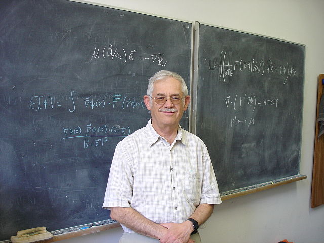
It’s time for me to write about physics again. I have a splendid reason: one of the recipients of this year’s physics Nobel is from Kingston, Ontario, which is practically in Ottawa’s backyard. He is recognized for his contribution to the discovery of neutrino oscillations. So I thought I’d write about neutrino oscillations a little.

Without getting into too much detail, the standard way of describing a theory of quantum fields is by writing down the so-called Lagrangian density of the theory. This Lagrangian density represents the kinetic and potential energies of the system, including so-called “mass terms” for fields that are massive. (Which, in quantum field theory, is the same as saying that the particles we associate with the unit oscillations of these fields have a specific mass.)

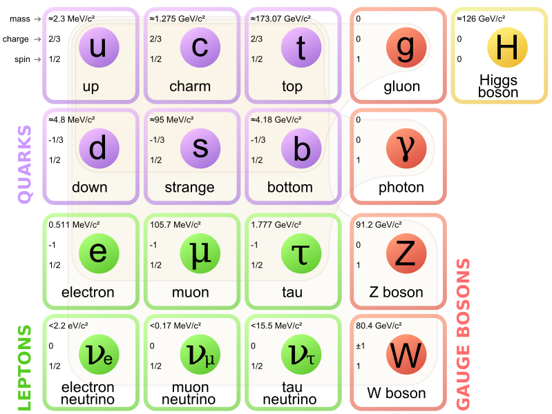
Now most massive particles in the Standard Model acquire their masses by interacting with the celebrated Higgs field in various ways. Not neutrinos though; indeed, until the mid 1990s or so, neutrinos were believed to be massless.

But then, neutrino oscillations were discovered and the physics community began to accept that neutrinos may be massive after all.

So what is this about oscillations? Neutrinos are somewhat complicated things, but I can demonstrate the concept using two hypothetical “scalar” particles (doesn’t matter what they are; the point is, their math is simpler than that of neutrinos.) So let’s have a scalar particle named $\phi$. Let’s suppose it has a mass, $\mu$. The mass term in the Lagrangian would actually be in the form, $\frac{1}{2}\mu\phi^2$.

Now let’s have another scalar particle, $\psi$, with mass $\rho$. This means another mass term in the Lagrangian: $\frac{1}{2}\rho\psi^2$.

But now I want to be clever and combine these two particles into a two-element abstract vector, a “doublet”. Then, using the laws of matrix multiplication, I could write the mass term as

$$\frac{1}{2}\begin{pmatrix}\phi&\psi\end{pmatrix}\cdot\begin{pmatrix}\mu&0\\0&\rho\end{pmatrix}\cdot\begin{pmatrix}\phi\\\psi\end{pmatrix}=\frac{1}{2}\mu\phi^2+\frac{1}{2}\rho\psi^2.$$

Clever, huh?

But now… let us suppose that there is also an interaction between the two fields. In the Lagrangian, this interaction would be represented by a term such as $\epsilon\phi\psi$. Putting $\epsilon$ into the “0” slots of the matrix, we get

$$\frac{1}{2}\begin{pmatrix}\phi&\psi\end{pmatrix}\cdot\begin{pmatrix}\mu&\epsilon\\\epsilon&\rho\end{pmatrix}\cdot\begin{pmatrix}\phi\\\psi\end{pmatrix}=\frac{1}{2}\mu\phi^2+\frac{1}{2}\rho\psi^2+\epsilon\phi\psi.$$

And here is where things get really interesting. That is because we can re-express this new matrix using a combination of a diagonal matrix and a rotation matrix (and its transpose):

$$\begin{pmatrix}\mu&\epsilon\\\epsilon&\rho\end{pmatrix}=\begin{pmatrix}\cos\theta/2&\sin\theta/2\\-\sin\theta/2&\cos\theta/2\end{pmatrix}\cdot\begin{pmatrix}\hat\mu&0\\0&\hat\rho\end{pmatrix}\cdot\begin{pmatrix}\cos\theta/2&-\sin\theta/2\\\sin\theta/2&\cos\theta/2\end{pmatrix},$$

which is equivalent to

$$\begin{pmatrix}\hat\mu&0\\0&\hat\rho\end{pmatrix}=\begin{pmatrix}\cos\theta/2&-\sin\theta/2\\\sin\theta/2&\cos\theta/2\end{pmatrix}\cdot\begin{pmatrix}\mu&\epsilon\\\epsilon&\rho\end{pmatrix}\cdot\begin{pmatrix}\cos\theta/2&\sin\theta/2\\-\sin\theta/2&\cos\theta/2\end{pmatrix},$$

$$\begin{pmatrix}\hat\mu&0\\0&\hat\rho\end{pmatrix}=\frac{1}{2}\begin{pmatrix}\mu+\rho+(\mu-\rho)\cos\theta-2\epsilon\sin\theta&(\rho-\mu)\sin\theta-2\epsilon\cos\theta\\(\rho-\mu)\sin\theta-2\epsilon\cos\theta&\mu+\rho+(\rho-\mu)\cos\theta+2\epsilon\sin\theta\end{pmatrix},$$

which tells us that $\tan\theta=2\epsilon/(\rho-\mu)$, which works so long as $\rho\ne\mu$.

Now why is this interesting? Because we can now write

\begin{align}\frac{1}{2}&\begin{pmatrix}\phi&\psi\end{pmatrix}\cdot\begin{pmatrix}\mu&\epsilon\\\epsilon&\rho\end{pmatrix}\cdot\begin{pmatrix}\phi\\\psi\end{pmatrix}\\
&{}=\frac{1}{2}\begin{pmatrix}\phi&\psi\end{pmatrix}\cdot\begin{pmatrix}\cos\theta/2&\sin\theta/2\\-\sin\theta/2&\cos\theta/2\end{pmatrix}\cdot\begin{pmatrix}\hat\mu&0\\0&\hat\rho\end{pmatrix}\cdot\begin{pmatrix}\cos\theta/2&-\sin\theta/2\\\sin\theta/2&\cos\theta/2\end{pmatrix}\cdot\begin{pmatrix}\phi\\\psi\end{pmatrix}\\
&{}=\frac{1}{2}\begin{pmatrix}\hat\phi&\hat\psi\end{pmatrix}\cdot\begin{pmatrix}\hat\mu&0\\0&\hat\rho\end{pmatrix}\cdot\begin{pmatrix}\hat\phi\\\hat\psi\end{pmatrix}.\end{align}

What just happened, you ask? Well, we just rotated the abstract vector $(\phi,\psi)$ by the angle $\theta/2$, and as a result, diagonalized the expression. Which is to say that whereas previously, we had two interacting fields $\phi$ and $\psi$ with masses $\mu$ and $\rho$, we now re-expressed the same physics using the two non-interacting fields $\hat\phi$ and $\hat\psi$ with masses $\hat\mu$ and $\hat\rho$.

So what is actually taking place here? Suppose that the doublet $(\phi,\psi)$ interacts with some other field, allowing us to measure the flavor of an excitation (particle) as being either a $\phi$ or a $\psi$. So far, so good.

However, when we attempt to measure the mass of the doublet, we will not measure $\mu$ or $\rho$, because the two states interact. Instead, we will measure $\hat\mu$ or $\hat\rho$, corresponding to the states $\hat\phi$ or $\hat\psi$, respectively: that is, one of the mass eigenstates.

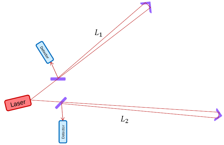
Which means that if we first perform a flavor measurement, forcing the particle to be in either the $\phi$ or the $\psi$ state, followed by a mass measurement, there will be a nonzero probability of finding it in either the $\hat\phi$ or the $\hat\psi$ state, with corresponding masses $\hat\mu$ or $\hat\rho$. Conversely, if we first perform a mass measurement, the particle will be either in the $\hat\phi$ or the $\hat\psi$ state; a subsequent flavor measurement, therefore, may give either $\phi$ or $\psi$ with some probability.

In short, the flavor and mass eigenstates do not coincide.

This is more or less how neutrino oscillations work (again, omitting a lot of important details), except things get a bit more complicated, as neutrinos are fermions, not scalars, and the number of flavors is three, not two. But the basic principle remains the same.

This is a unique feature of neutrinos, by the way. Other particles, e.g., charged leptons, do not have mass eigenstates that are distinct from their flavor eigenstates. The mechanism that gives them masses is also different: instead of a self-interaction in the form of a mass matrix, charged leptons (as well as quarks) obtain their masses by interacting with the Higgs field. But that is a story for another day.

Featured on XKCD

Personal, Physics, Pop culture, Space No Responses »

Aug 282015

Hey, I just noticed that our resolution of the Pioneer anomaly made it to an xkcd comic:

Wow. Who knows, if things continue like this, we might even end up on The Simpsons or The Big Bang Theory.

Jacob Bekenstein

Physics No Responses »

Aug 182015

I woke up this morning to the news that Mexican-Israeli physicist Jacob Bekenstein died two days ago, at the age of 68, in Helsinki, Finland. I saw nothing about the cause of death.

Bekenstein’s work is well known to folks dealing with gravity theory. Two of his contributions stand out in particular.

First, Bekenstein was first to suggest that black holes should have entropy. His work, along with that of Stephen Hawking, led to the Bekenstein-Hawking entropy formula $S=kc^3A/4G\hbar$, relating the black hole’s surface area $A$ to its entropy $S$ using the speed of light $c$, the gravitational constant $G$, the reduced Planck constant $\hbar$ and Boltzmann’s constant $k$. With this work, the science of black hole thermodynamics was born, leading to all kinds of questions about the nature of black holes and the connection between thermodynamics and gravity, many of which remain unanswered to this day.

Bekenstein’s second contribution was to turn Morehai Milgrom’s MOdified Newtonian Dynamics (MOND) into a respectable relativitistic theory. The MOND paradigm is about replacing Newton’s law relating force $({\mathbf F})$, mass $(m)$ and acceleration $({\mathbf a})$, ${\mathbf F}=m{\mathbf a}$, with the modified law ${\mathbf F}=\mu(a/a_0)m{\mathbf a}$, where all we know about the function $\mu(x)$ is that $\lim_{x\to 0}\mu(x)=x$ and $\lim_{x\to\infty}\mu(x)=1$. Surprisingly, the right choice of $a_0$ results in an acceleration law that explains the anomalous rotation of galaxies without the need for dark matter. However, in this form, MOND is theoretically ugly: it is a formula that violates basic conservation laws, including the consevation of energy, for instance. Bekenstein’s TeVeS (Tensor-Vector-Scalar) gravity theory provides a general relativistic framework for MOND, one that does respect basic conservation laws, yet reproduces the MOND acceleration formula in the low energy limit.

I never met Jacob Bekenstein, and now I never will. A pity. May he rest in peace.

Light echo

Astronomy, Physics No Responses »

Aug 032015

Here is one of the most mind-boggling animation sequences that I have ever seen:

This image depicts V838 Monocerotis, a red variable star that underwent a major outburst back in 2002.

Why do I consider this animation mind-boggling? Because despite all appearances, it is not an expanding shell of dust or gas.

Rather, it is echoes of the flash of light, reflected by dust situated behind the star, reaching our eyes several years after the original explosion.

In other words, this image represents direct, visual evidence of the finite speed of light.

The only comparable thing that I can think of is this video, created a few years ago using tricky picosecond photography, of a laser pulse traveling in a bottle. However, unlike that video, the images of V838 Monocerotis required no trickery, only a telescope.

And light echoes are more than mere curiosities: they actually make it possible to study past events. Most notably, a faint light echo of a supernova that was observed nearly half a millennium ago, in 1572, was detected in 2008.

Building a quantum theory

Physics No Responses »

Jul 202015

$\renewcommand{\vec}[1]{\boldsymbol{\mathrm{#1}}}$Continuing something I began about a month ago, I spent more of my free time than I care to admit re-deriving some of the most basic identities in quantum physics.

I started with the single-particle case of a harmonic oscillator. Such an oscillator is characterized by the classical Lagrangian

$$L=\frac{1}{2}m\dot{\vec{q}}^2-\frac{1}{2}k\vec{q}^2-V(\vec{q}),$$

and the corresponding Hamiltonian

$$H=\frac{\vec{p}^2}{2m}+\frac{1}{2}k\vec{q}^2+V(\vec{q}).$$

By multiplying this Hamiltonian with $\psi=e^{i(\vec{p}\cdot\vec{q}-Ht)/\hbar}$, we basically obtain Schrödinger’s equation:

$$\left[i\hbar\partial_t+\frac{\hbar^2}{2m}\vec{\nabla}^2-\frac{1}{2}k\vec{q}^2-V(\vec{q})\right]e^{i(\vec{p}\cdot\vec{q}-Ht)/\hbar}=0.$$

The transition to the quantum theory begins when we accept that linear combinations of solutions of this equation (i.e., $\psi$-s corresponding to different values of $\vec{p}$ and $H$) also represent physical states of the system, despite the fact that these “mixed” solutions are not eigenfunctions and there are no corresponding classical eigenvalues $\vec{p}$ and $H$.

Pure algebra can lead to an expression of $\hat{H}$ in the form of “creation” and “annihilation” operators:

$$\hat{H}=\hbar\omega\left(\hat{a}^\dagger\hat{a}+\frac{1}{2}\right)+V(\vec{q}).$$

These operators have the properties

\begin{align*}
\hat{H}\hat{a}\psi_n&=\left([\hat{H},\hat{a}]+\hat{a}\hat{H}\right)\psi_n=(E_n-\hbar\omega)\hat{a}\psi_n,\\
\hat{H}\hat{a}^\dagger\psi_n&=\left([\hat{H},\hat{a}^\dagger]+\hat{a}^\dagger\hat{H}\right)\psi_n=(E_n+\hbar\omega)\hat{a}^\dagger\psi_n.
\end{align*}
where

$$E_n=\left(n+\frac{1}{2}\right)\hbar\omega.$$

This same derivation can be done in the relativistic single particle case as well.

Moreover, it is possible to define a classical scalar field in the form

$${\cal L}=\frac{1}{2}\rho(\partial_t\phi)^2-\frac{1}{2}\rho c^2(\vec{\nabla}\phi)^2-\frac{1}{2}\kappa\phi^2-V(\phi),$$

which leads to the Hamiltonian density

$${\cal H}=\pi\partial_t\phi-{\cal L}=\frac{\pi^2}{2\rho}+\frac{1}{2}\rho c^2(\vec{\nabla}\phi)^2+\frac{1}{2}\kappa\phi^2+V(\phi).$$

The transitioning to the quantum theory occurs by first expressing $\phi$ as a Fourier integral and then promoting the Fourier coefficients to operators that satisfy a commutation relation in the form

$$[\hat{a}(\omega,\vec{k}),\hat{a}^\dagger(\omega,\vec{k}’)]=(2\pi)^3\delta^3(\vec{k}-\vec{k}’).$$

This leads to a commutation relation for the field and its canonical momentum in the form

$$[\hat{\phi}(t,\vec{x}),\hat{\pi}(t,\vec{x}’)]=i\hbar\delta^3(\vec{x}-\vec{x}’),$$

and for the Hamiltonian,

$$\hat{H}=\hbar\omega\left\{\frac{1}{2}+\int\frac{d^3\vec{k}}{(2\pi)^3}\hat{a}^\dagger(\omega,\vec{k})\hat{a}(\omega,\vec{k})\right\}+\int d^3xV(\hat{\phi}).$$

More details are provided on my Web site, at https://www.vttoth.com/CMS/physics-notes/297.

So why did I find it necessary to capture here something that can be found in first chapter of every semi-decent quantum field theory textbook? Several reasons.

First, I wanted to present a consistent treatment of all four cases: the nonrelativistic and relativistic case for both the particle and the field theory.
Second, I wanted to write down all relevant equations without omitting dimensions. I wanted to write down a Lagrangian density that has the dimensions of energy density, consistent with a scalar field that has the dimensions of length (i.e., a displacement).
Third, I wanted to spell out some of the details of the derivation that are omitted from nearly all textbooks yet, I am obliged to admit, almost stumped me. That is, once you see the derivation the steps are reasonably trivial, but it is still hard to stumble upon exactly the right way to apply the relevant identities related to Fourier transforms and Dirac deltas.
Lastly, I find it revealing how this approach can highlight exactly where a quantum theory is introduced. In the particle theory case, it is when we assume that “mixed states”, that is, linear combinations of eigenstates also represent physical states of a system, despite the fact that they do not correspond to classical eigenvalues. In the case of a field theory, the transition occurs when we replace Fourier coefficients with operators: implicit in the transition is that once again, mixed states are included as representing actual physical states of the system.

Note also how none of this has anything to do with interpretations. There is no “collapse of the wave function” or any such nonsense. That stuff happens when we introduce into our consideration a “measurement event”, effectively an interaction between the quantum system and a classical instrument, which forces the quantum system into an eigenstate. This eigenstate cannot be predicted from the initial conditions alone, precisely because the classical idealization of the measurement apparatus effectively amounts to an admission of ignorance about its true quantum state.

How to derive Schrödinger’s equation

Physics No Responses »

Jun 212015

There is a particularly neat way to derive Schrödinger’s equation, and to justify the “canonical substitution” rules for replacing energy and momentum with corresponding operators when we “quantize” an equation.

Take a particle in a potential. Its energy is given by

$$E=\frac{{\bf p}^2}{2m}+V({\bf x}),$$

$$E-\frac{{\bf p}^2}{2m}-V({\bf x})=0.$$

Now multiply both sides this equation by the formula $e^{i({\bf p}\cdot{\bf x}-Et)/\hbar}$. We note that this exponential expression cannot ever be zero if the part in the exponent that’s in parentheses is real:

$$\left[E-\frac{{\bf p}^2}{2m}-V({\bf x})\right]e^{i({\bf p}\cdot{\bf x}-Et)/\hbar}=0.$$

So far so good. But now note that

$$Ee^{i({\bf p}\cdot{\bf x}-Et)/\hbar}=i\hbar\frac{\partial}{\partial t}e^{i({\bf p}\cdot{\bf x}-Et)/\hbar},$$

and similarly,

$${\bf p}^2e^{i({\bf p}\cdot{\bf x}-Et)/\hbar}=-\hbar^2{\boldsymbol\nabla}e^{i({\bf p}\cdot{\bf x}-Et)/\hbar}.$$

This allows us to rewrite the previous equation as

$$\left[i\hbar\frac{\partial}{\partial t}+\hbar^2\frac{{\boldsymbol\nabla}^2}{2m}-V({\bf x})\right]e^{i({\bf p}\cdot{\bf x}-Et)/\hbar}=0.$$

Or, writing $\Psi=e^{i({\bf p}\cdot{\bf x}-Et)/\hbar}$ and rearranging:

$$i\hbar\frac{\partial}{\partial t}\Psi=-\hbar^2\frac{{\boldsymbol\nabla}^2}{2m}\Psi+V({\bf x})\Psi,$$

which is the good old Schrödinger equation.

The method works for an arbitrary, generic Hamiltonian, too. Given

$$H({\bf p})=E,$$

we can write

$$\left[E-H({\bf p})\right]e^{i({\bf p}\cdot{\bf x}-Et)/\hbar}=0,$$

which is equivalent to

$$\left[i\hbar\frac{\partial}{\partial t}-H(-i\hbar{\boldsymbol\nabla})\right]\Psi=0.$$

So if this equation is identically satisfied for a classical system with Hamiltonian $H$, what’s the big deal about quantum mechanics? Well… a classical system satisfies $E-H({\bf p})=0$, where $E$ and ${\bf p}$ are eigenvalues of the differential operators $i\hbar\partial/\partial t$ and $-i\hbar{\boldsymbol\nabla}$, respectively. Schrödinger’s equation, on the other hand, remains valid in the general case, not just for the eigenvalues.

A small honor

Personal, Physics No Responses »

Mar 242015

The editors of Physical Review D decided that our paper about the stability of boson condensate stars: specifically, a diagram that shows 36 simulated cases, deserves to be featured on their new Kaleidoscope page for February 2015:

Thank you, Physical Review.

Emmy Noether’s birthday

History, Internet, Physics No Responses »

Mar 232015

Emmy Noether… not exactly a household name, at least outside of the community of theoretical physicists and mathematicians.

Which is why I was so surprised today when I noticed Google’s March 23 Doodle: a commemoration of Emmy Noether’s 133rd birthday.

Wow. I mean, thank you, Google. What a nice and deserving tribute to one of my heroes.

Two papers

Personal, Physics 1 Response »

Mar 052015

Last month, something happened to me that may never happen again: I had not one but two papers accepted by Physical Review D in the same month, on two completely different topics.

The first was a paper I wrote with John Moffat, showing how well his scalar-tensor-vector gravity theory (STVG, also called MOG) fits an extended set of Milky Way rotational curve data out to a radius of nearly 200 kpc. In contrast, the archetypal modified gravity theory, MOND (Mordehai Milgrom’s MOdified Newtonian Dynamics) does not fare so well: as it predicts a flat rotation curve, its fit to the data is rather poor, although its advocates suggest that the fit might improve if we take into account the “external” gravitational field due to other galaxies.

The other paper, which I wrote together with an old friend and colleague, Eniko Madarassy, details a set of numerical simulations of self-gravitating Bose-Einstein condensates, which may form exotic stars or stellar cores. There has been some discussion in the literature concerning the stability of such objects. Our simulation shows that they are stable, which confirms my own finding, detailed in an earlier paper (which, curiously, was rejected by PRD), namely that the perceived instability arises from an inappropriate application of an approximation (the Thomas-Fermi approximation) used to provide a simplistic description of the condensate.

Oh, and we also had another paper accepted, not by Physical Review D, but by the International Journal of Modern Physics D, but still… it is about yet another topic, post-Galilean coordinate transformations and the analysis of the N-body problem in general relativity. Unlike the first two papers, this one was mostly the work of my co-author, Slava Turyshev, but I feel honored to have been able to contribute. It is a 48-page monster (in the rather efficient REVTeX style; who knows how many pages it will be in the style used by IJMPD) with over 400 equations.

All in all, a productive month insofar as my nonexistent second career as a theoretical physicist is concerned. Now I have to concentrate on my first job, the one that feeds the cats…

Quantum physics poll

Physics No Responses »

Feb 082015

cat-dead-alive I have some half-baked ideas about the foundations of quantum physics (okay, who doesn’t.) When I say half-baked, I don’t mean that they are stupid (I sure hope not!) I simply mean I am not 100% sure about them, and there is more to learn.

But, I am allowed to have opinions. So when I came across this informal 2013 poll among (mostly) quantum physicists, I decided to answer the questions myself.

Question 1: What is your opinion about the randomness of individual quantum events (such as the decay of a radioactive atom)?

a. The randomness is only apparent: 9%
b. There is a hidden determinism: 0%
c. The randomness is irreducible: 48%
d. Randomness is a fundamental concept in nature: 64%

(“Jedenfalls bin ich überzeugt, daß [der Alte] nicht würfelt.”)

Question 2: Do you believe that physical objects have their properties well defined prior to and independent of measurement?

a. Yes, in all cases: 3%
b. Yes, in some cases: 52%
c. No: 48%
d. I’m undecided: 9%

(Note that the question does not say that “well-defined” is a synonym for “in an eigenstate”.)

Question 3: Einstein’s view of quantum mechanics

a. Is correct: 0%
b. Is wrong: 64%
c. Will ultimately turn out to be correct: 6%
d. Will ultimately turn out to be wrong: 12%
e. We’ll have to wait and see: 12%

(Einstein’s views are dated, but I feel that he may nonetheless be vindicated because his reasons for holding those views would turn out to be valid. But, we’ll have to wait and see.)

Question 4: Bohr’s view of quantum mechanics

a. Is correct: 21%
b. Is wrong: 27%
c. Will ultimately turn out to be correct: 9%
d. Will ultimately turn out to be wrong: 3%
e. We’ll have to wait and see: 30%

(If I said “wait and see” on Einstein’s views, how could I possibly answer this question differently?)

Question 5: The measurement problem

a. A pseudoproblem: 27%
b. Solved by decoherence: 15%
c. Solved/will be solved in another way: 39%
d. A severe difficulty threatening quantum mechanics: 24%
e. None of the above: 27%

(Of course it’s a pseudoproblem. It vanishes the moment you look at the whole world as a quantum world.)

Question 6: What is the message of the observed violations of Bell’s inequalities?

a. Local realism is untenable: 64%
b. Action-at-a-distance in the physical world: 12%
c. Some notion of nonlocality: 36%
d. Unperformed measurements have no results: 52%
e. Let’s not jump the gun—let’s take the loopholes more seriously: 6%

(I don’t like how the phrase “local realism” is essentially conflated with classical eigenstates. Why is a quantum state not real?)

Question 7: What about quantum information?

a. It’s a breath of fresh air for quantum foundations: 76%
b. It’s useful for applications but of no relevance to quantum foundations: 6%
c. It’s neither useful nor fundamentally relevant: 6%
d. We’ll need to wait and see: 27%

(I wish there was another option: e. A fad. Then again, it does have some practical utility, so b is my answer.)

Question 8: When will we have a working and useful quantum computer?

a. Within 10 years: 9%
d. In 10 to 25 years: 42%
c. In 25 to 50 years: 30%
d. In 50 to 100 years: 0%
e. Never: 15%

(The threshold theorem supposedly tells us what it takes to avoid decoherence. What I think it tells us is the limits of quantum error correction and why decoherence is unavoidable.)

Question 9: What interpretation of quantum states do you prefer?

a. Epistemic/informational: 27%
b. Ontic: 24%
c. A mix of epistemic and ontic: 33%
d. Purely statistical (e.g., ensemble interpretation): 3%
e. Other: 12%

(Big words look-up time, but yes, ontic it is. I may have remembered the meaning of “ontological”, but I nonetheless would have looked up both, just to be sure that I actually understand how these terms are used in the quantum physics context.)

Question 10: The observer

a. Is a complex (quantum) system: 39%
b. Should play no fundamental role whatsoever: 21%
c. Plays a fundamental role in the application of the formalism but plays no distinguished physical role: 55%
d. Plays a distinguished physical role (e.g., wave-function collapse by consciousness): 6%

(Of course the observer is a complex quantum system. I am surprised that some people still believe this new age quantum consciousness bull.)

Question 11: Reconstructions of quantum theory

a. Give useful insights and have superseded/will supersede the interpretation program: 15%
b. Give useful insights, but we still need interpretation: 45%
c. Cannot solve the problems of quantum foundations: 30%
d. Will lead to a new theory deeper than quantum mechanics: 27%
e. Don’t know: 12%

(OK, I had to look up the papers, as I had no recollection of the word “reconstruction” used in this context. As it turns out, I’ve seen papers in the past on this topic and they left me unimpressed. My feeling is that even as they purport to talk about quantum theory, what they actually talk about are (some of) its interpretations. And all too often, people who do this leave QFT completely out of the picture, even though it is a much more fundamental theory than single particle quantum mechanics!)

Question 12: What is your favorite interpretation of quantum mechanics?

a. Consistent histories: 0%
b. Copenhagen: 42%
c. De Broglie–Bohm: 0%
d. Everett (many worlds and/or many minds): 18%
e. Information-based/information-theoretical: 24%
f. Modal interpretation: 0%
g. Objective collapse (e.g., GRW, Penrose): 9%
h. Quantum Bayesianism: 6%
i. Relational quantum mechanics: 6%
j. Statistical (ensemble) interpretation: 0%
k. Transactional interpretation: 0%
l. Other: 12%
m. I have no preferred interpretation 12%

(OK, this is the big one: which camp is yours! And the poll authors themselves admit that it was a mistake to leave out n. Shut up and calculate. I am disturbed by the number of people who opted for Everett. Information-based interpretations seem to be the fad nowadays. I am surprised by the complete lack of support for the transactional interpretation, and also by the low level of support for Penrose. I put myself in the Other category, because my half-baked ideas don’t precisely fit into any of these boxes.)

Question 13: How often have you switched to a different interpretation?

a. Never: 33%
b. Once: 21%
c. Several times: 21%
d. I have no preferred interpretation: 21%

(I am not George W. Bush. I don’t “stay the course”. I change my mind when I learn new things.)

Question 14: How much is the choice of interpretation a matter of personal philosophical prejudice?

a. A lot: 58%
b. A little: 27%
c. Not at all: 15%

(I put my mark on a. because that’s the way it is today. If you asked me how it should be, I’d have answered c.)

Question 15: Superpositions of macroscopically distinct states

a. Are in principle possible: 67%
b. Will eventually be realized experimentally: 36%
c. Are in principle impossible: 12%
d. Are impossible due to a collapse theory: 6%

(Of course it’s a. Quantum physics is not about size, it’s about the number of independent degrees of freedom.)

Question 16: In 50 years, will we still have conferences devoted to quantum foundations?

a. Probably yes: 48%
b. Probably no: 15%
c. Who knows: 24%
d. I’ll organize one no matter what: 12%

(Probably yes but do I really care?)

OK, now that I answered these poll questions myself, does that make me smart? I don’t feel any smarter.

The Paks nuclear incident

Hungary, Physics No Responses »

Jan 042015

Courtesy to a two-part article (part 1 and part 2, in Hungarian) of the Hungarian satirical-liberal magazine Magyar Narancs (Hungarian Orange), I now have a much better idea of what happened at Hungary’s sole nuclear generating station, the Paks Nuclear Power Plant, in 2003. It was the most serious nuclear incident to date in Hungary (the only INES level 3 incident in the country.)

At the root of the incident is a characteristic issue with these types of Soviet era nuclear reactors leading to magnetite contamination of the fuel elements and control rods. To deal with this contamination and prolong the life of fuel elements, cleaning ponds are installed next to the reactor blocks, where under roughly 30 feet of water, in a specially designed cleaning tank, fuel bundles can be cleaned.

As the problem of contamination became increasingly acute, the power plant ordered a new type of cleaning tank. On April 10, 2003, this cleaning tank was used for the first time on fuel bundles that were freshly removed from the reactor. The cleaning of the fuel bundles was completed successfully by 5 PM in the afternoon; however, the crane that was supposed to replace the fuel bundle in the reactor was used for another task and was not going to be available before midnight. The situation was complicated by language issues, as the technicians attending the new cleaning tank were from Germany and could not speak Hungarian. Nonetheless, the German crew assured the plant’s management that the delay would not represent a problem and that cooling of the fuel bundle inside the cleaning tank was adequate.

Shortly before 10 PM, an alarm system detected increased radiation and noble gas levels in the hall housing the cleaning pond. Acting upon the suspicion that a fuel rod assembly was leaking (the German crew suggested that the fuel bundles may have been incorrectly placed in the cleaning tank) the crew proceeded with a plan to open the cleaning tank. When the lid of the cleaning vessel was unlocked, a large steam bubble was released, and radiation levels spiked. Indeed, the crane operator received a significant dose of radiation contamination on his face and arms. The hall was immediately evacuated and its ventilation system was turned on. However, as the system had no adequate filtering systems installed (despite a regulation that six years prior mandated their installation) some radiation was released into the environment.

As it turns out, the culprit was the new type of cleaning tank. A model that, incidentally, was approved using an expedited process, due to the urgency of the situation at the power plant. The fact that the supplier was a proven entity also contributed to a degree of complacency.

Both the new and the old tank had a built-in pump that circulated water and kept the fuel bundle cool. However, in the old tank, the water inlet was at the bottom, whereas the outlet was near the top. This was not the case in the new tank: both inlet and outlet were located at the bottom, which allowed the formation of steam inside the cleaning vessel near the top. Combined with the lack of instrumentation, and considering that the fuel bundle released as much as 350 kW of heat, this was a disaster in the making.

And that is exactly what happened: due to the delay with the crane, there was enough time for the heat from the fuel bundle to cause most of the water inside the vessel to turn into steam, and the fuel elements heated to 1,000 degrees Centigrade. This caused their insulation to crack, which led to the initial detection of increased radiation levels. When the cleaning tank’s lid was opened, a large bubble of steam was released, while cold water rushed in causing a minor steam explosion and breaking up the fuel elements inside, contaminating the entire pond.

It took another ten years before the last remaining pieces of broken-up fuel elements were removed from the power plant, taken by train through Ukraine to a reprocessing plant in Russia. The total cost of the incident was in the $100 million range.

As nuclear incidents go, Paks was by no means among the scariest: after all, no lives were lost, there was only one person somewhat contaminated, and there was negligible environmental damage. This was no Chernobyl, Fukushima or Three Mile Island. There was some economic fallout, as this reactor block remained inoperative for about a year, but that was it.

Nonetheless, this incident is yet another example how inattention by regulatory agencies, carelessness, or failure to adhere to regulations can lead to catastrophic accidents. Despite its reputation, nuclear power remains one of the safest (and cleanest!) ways to generate electricity but, as engineers are fond of saying, there are no safeguards against human stupidity.

The parameters of the Standard Model

Physics 1 Response »

Nov 042014

Many popular science books and articles mention that the Standard Model of particle physics, the model that unifies three of the fundamental forces and describes all matter in the form of quarks and leptons, has about 18 free parameters that are not predicted by the theory.

Very few popular accounts actually tell you what these parameters are.

So here they are, in no particular order:

The so-called fine structure constant, $\alpha$, which (depending on your point of view) defines either the coupling strength of electromagnetism or the magnitude of the electron charge;
The Weinberg angle or weak mixing angle $\theta_W$ that determines the relationship between the coupling constant of electromagnetism and that of the weak interaction;
The coupling constant $g_3$ of the strong interaction;
The electroweak symmetry breaking energy scale (or the Higgs potential vacuum expectation value, v.e.v.) $v$;
The Higgs potential coupling constant $\lambda$ or alternatively, the Higgs mass $m_H$;
The three mixing angles $\theta_{12}$, $\theta_{23}$ and $\theta_{13}$ and the CP-violating phase $\delta_{13}$ of the Cabibbo-Kobayashi-Maskawa (CKM) matrix, which determines how quarks of various flavor can mix when they interact;
Nine Yukawa coupling constants that determine the masses of the nine charged fermions (six quarks, three charged leptons).

OK, so that’s the famous 18 parameters so far. It is interesting to note that 15 out of the 18 (the 9 Yukawa fermion mass terms, the Higgs mass, the Higgs potential v.e.v., and the four CKM values) are related to the Higgs boson. In other words, most of our ignorance in the Standard Model is related to the Higgs.

Beyond the 18 parameters, however, there are a few more. First, $\Theta_3$, which would characterize the CP symmetry violation of the strong interaction. Experimentally, $\Theta_3$ is determined to be very small, its value consistent with zero. But why is $\Theta_3$ so small? One possible explanation involves a new hypothetical particle, the axion, which in turn would introduce a new parameter, the mass scale $f_a$ into the theory.

Finally, the canonical form of the Standard Model includes massless neutrinos. We know that neutrinos must have mass, and also that they oscillate (turn into one another), which means that their mass eigenstates do not coincide with their eigenstates with respect to the weak interaction. Thus, another mixing matrix must be involved, which is called the Pontecorvo-Maki-Nakagawa-Sakata (PMNS) matrix. So we end up with three neutrino masses $m_1$, $m_2$ and $m_3$, and the three angles $\theta_{12}$, $\theta_{23}$ and $\theta_{13}$ (not to be confused with the CKM angles above) plus the CP-violating phase $\delta_{\rm CP}$ of the PMNS matrix.

So this is potentially as many as 26 parameters in the Standard Model that need to be determined by experiment. This is quite a long way away from the “holy grail” of theoretical physics, a theory that combines all four interactions, all the particle content, and which preferably has no free parameters whatsoever. Nonetheless the theory, and the level of our understanding of Nature’s fundamental building blocks that it represents, is a remarkable intellectual achievement of our era.

Feynman’s lectures online

Physics No Responses »

Sep 042014

Richard Feynman’s Lectures on Physics remains a classic to this day.

Its newest edition has recently (I don’t know exactly when, I only came across it a few days ago) been made available in its entirety online, for free. It is a beautifully crafted, very high quality online edition, using LaTeX (MathJax) for equations, redrawn scalable figures.

Perhaps some day, someone will do the same to Landau’s and Lifshitz’s 10-volume Theoretical Physics series, too?

Einstein’s field equations… in a Subway sandwich commercial?

Physics, Television No Responses »

Aug 132014

Last night, as I was watching the latest episode of Tyrant (itself an excellent show about a fictitious Middle Eastern dictatorship and its ruling family), I happened to glance at the TV during a commercial break just at the right split second to see this:

This was part of an ad, a Subway sandwich commercial, with an animated monkey handing this exam sheet back to a student (also a monkey). What caught my eye was the equation on this sheet. What??? Einstein’s field equations?

Yup, that’s exactly what I saw there, the equation $G_{\alpha\beta}=\dfrac{8\pi G}{c^4}T_{\alpha\beta}$. General relativity.

Other, easily recognizable equations on the sheet included an equation of the electrostatic Coulomb force, the definition of the quantum mechanical probability amplitude, and the continuity equation.

What struck me was that all these are legitimate equations from physics, not gibberish. And all that in a silly Subway commercial. Wow.

Planck length physics

Physics No Responses »

Apr 042014

A physics meme is circulating on the Interwebs, suggesting that any length shorter than the so-called Planck length makes “no physical sense”.

Which, of course, is pure nonsense.

The Planck length is formed using the three most fundamental constants in physics: the speed of light, $c = 3\times 10^8~{\rm m}/{\rm s}$; the gravitational constant, $G = 6.67\times 10^{-11}~{\rm m}^3/{\rm kg}\cdot{\rm s}^2$; and the reduced Planck constant, $\hbar = h/2\pi = 1.05\times 10^{-34}~{\rm m}^2{\rm kg}/{\rm s}$.

Of these, the speed of light just relates two human-defined units: the unit of length and the unit of time. Nothing prevents us from using units in which $c = 1$; for instance, we could use the second as our unit of time, and the light-second ($= 300,000~{\rm km}$) as our unit of length. In other words, the expression $c = 300,000,000~{\rm m}/{\rm s}$ is just an instruction to replace every occurrence of the symbol ${\rm s}$ with the quantity $300,000,000~{\rm m}$.

If we did this in the definition of $G$, we get a new value: $G’ = G/c^2 = 7.41\times 10^{-28}~{\rm m}/{\rm kg}$.

Splendid, because this reveals that the gravitational constant is also just a relationship between human-defined units: the unit of length vs. the unit of mass. It allows us to replace every occurrence of the symbol ${\rm kg}$ with the quantity $7.41\times 10^{-28}~{\rm m}$.

So let’s do this to the reduced Planck constant: $\hbar’ = \hbar G/c^3 = 2.61\times 10^{-70}~{\rm m}^2$. This is not a relationship between two human-defined units. This is a unit of area. Arguably, a natural unit of area. Taking its square root, we get what is called the Planck length: $l_P = 1.61\times 10^{-35}~{\rm m}$.

The meme suggests that a distance less than $l_P$ has no physical meaning.

But then, take two gamma rays, with almost identical energies, differing in wavelength by one Planck length, or about $10^{-35}~{\rm m}$.

Suppose these gamma rays originate from a spacecraft one astronomical unit (AU), or about $1.5\times 10^{11}~{\rm m}$ from the Earth.

The wavelength of a modest, $1~{\rm MeV}$ gamma ray is about $1.2\times 10^{-12}~{\rm m}$.

The number of full waves that fit in a distance of $1.5\times 10^{11}~{\rm m}$ is, therefore, is about $1.25\times 10^{23}$ waves.

A difference of $10^{-35}~{\rm m}$, or one Planck length, in wavelength adds up to a difference of $1.25\times 10^{-12}~{\rm m}$ over the $1~{\rm AU}$ distance, or more than one full wavelength of our gamma ray.

In other words, a difference of less than one Planck length in wavelength between two gamma rays is quite easily measurable in principle.

In practice, of course we’d need stable gamma ray lasers placed on interplanetary spacecraft and a sufficiently sensitive gamma ray interferometer, but nothing in principle prevents us from carrying out such a measurement, and all the energy, distance, and time scales involved are well within accessible limits at present day technology.

And if we used much stronger gamma rays, say at the energy level of the LHC (which is several million times more powerful), a distance of only a few thousand kilometers would be sufficient to detect the interference.

So please don’t tell me that a distance less than one Planck length has no physical meaning.

CERN to switch to Comic Sans for good

Physics No Responses »

Apr 012014

When the European Organization for Nuclear Research, better known by its French acronym as CERN, presented their finding of the Higgs boson in the summer of 2012, the world was most impressed by their decision to show slides prepared using the whimsical Comic Sans typeface.

Emboldened by their success, CERN today announced that as of April 1, 2014, all official CERN communication channels will switch to use Comic Sans exclusively.

Tensor modes, scalar modes and inflation

Physics No Responses »

Mar 182014

So the big announcement was made yesterday: r = 0.2. The inflationary Big Bang scenario is seemingly confirmed.

If confirmed, this discovery is of enormous significance. (Of course, extraordinary claims require extraordinary evidence.)

So here is the thing. In gravity, just as in electromagnetism, outside of a spherically symmetric body, the field will be indistinguishable from that of a point source. So for instance, if the Earth were a perfect sphere, simply by looking at the orbit of the Moon, you could not possible tell if the Earth was tiny and superdense, or large and less dense… only that its total mass is roughly six quadrillion kilograms.

A consequence of this is that if a spherically symmetric body expands and contracts, its (electrical or gravitational) field does not change. In other words, there is no such thing as monopole radiation.

In the case of electromagnetism, we can separate positive and negative charges. Crudely speaking, this is what a transmitting antenna does… and as a result, it produces dipole radiation. However, there is no such thing as negative mass: hence, there is no such thing is dipole gravitational radiation.

The next thing happens when you take a spherically symmetric body and squeeze it in one direction while allowing it to expand in the other. When you do this, the (electric or gravitational) field of the body will change. These changes will propagate in the form of quadrupole radiation. This is the simplest form of gravitational waves that there is. This method of generating radiation is very inefficient… which is one of the reasons why gravitational waves are both hard to produce and hard to detect.

To date, nobody detected gravitational waves directly. However, we did detect changes in the orbital periods of binary pulsars (superdense stars orbiting each other in very tight orbits) that is consistent with the loss of kinetic energy due to gravitational radiation.

Gravitational radiation was also produced when the Universe was very young, very dense, expanding rapidly. One particular theory of the early expansion is the inflationary theory, which suggests that very early, for a short time the Universe underwent extremely rapid expansion. This may explain things such as why the observable Universe is as homogeneous, as “flat” as it appears to be. This extremely rapid expansion would have produced strong gravitational waves.

Our best picture of the early Universe comes from our observations of the cosmic microwave background: leftover light from when the Universe was about 380,000 years old. This light, which we see in the form of microwave radiation, is extremely smooth, extremely uniform. Nonetheless, its tiny bumps already tell us a great deal about the early Universe, most notably how structures that later became planets and stars and galaxies began to form.

This microwave radiation, like all forms of electromagnetic radiation including light, can be polarized. Normally, you would expect the polarization to be random, a picture kind of like this one:

However, the early Universe already had areas that were slightly denser than the rest (these areas were the nuclei around which galaxies later formed.) Near such a region, the polarization is expected to line up preferably in the direction of the excess density, perhaps a little like this picture:

This is called the scalar mode or E-mode.

Gravitational waves can also cause the polarization of microwaves to line up, but somewhat differently, introducing a twist if you wish. This so-called tensor mode or B-mode pattern will look more like this:

We naturally expect to see B-modes as a result of the early expansion. We expect to see an excess of B-modes if the early expansion was governed by inflation.

And this is exactly what the BICEP2 experiment claims to have found. The excess is characterized by the tensor-to-scalar ratio, r = 0.2, and they claim it is a strong, five-sigma result.

Two questions were raised immediately concerning the validity of this result. First, why was this not detected earlier by the Planck satellite? Well, according to the paper and the associated FAQ, Planck only observed B-modes indirectly (inferred from temperature fluctuation measurements) and in any case, the tension between the two results is not that significant:

The other concern is that they seem to show an excess at higher multipole moments. This may be noise, a statistical fluke, or an indication of an unmodeled systematic that, if present, may degrade or even wipe out the claimed five sigma result:

speccomp

The team obviously believes that their result is robust and will withstand scrutiny. Indeed, they were so happy with the result that they decided to pay a visit to Andrei Linde, one of the founding fathers, if you wish, of inflationary cosmology:

What can I say? I hope there will be no reason for Linde’s genuine joy to turn into disappointment.

As to the result itself… apparent confirmation of a prediction of the inflationary scenario means that physical cosmology has reached the point where it can make testable predictions about the Universe when its age, as measured from the Big Bang, was less than one one hundredth of a quintillionth of a second. That is just mind-bogglingly insane.

Concave telescope

Physics No Responses »

Feb 182014

I don’t normally comment on crank science that finds its way into my Inbox, but this morning I got a really good laugh.

The announcement was dramatic enough: the e-mail bore the title, “Apparent detection of antimatter galaxies”. It came from the “Santilli foundation”, who sent me some eyebrow-raising e-mails in the past, but this was sufficiently intriguing to make me click on the link they provided. So click I did, only to be confronted with the following image:

What’s that, you ask? Why, a telescope with a concave lens. Had I paid a little bit more attention to the e-mail, I might have been a little less surprised; they did include a longer title, you see, helpfully typeset in all caps, which read, “APPARENT DETECTION OF ANTIMATTER GALAXIES VIA SANTILLI’S TELESCOPE WITH CONCAVE LENSES”.

Say what? Concave lenses? Why, it’s only logical. If light from an ordinary galaxy is focused by a convex lens, then surely, light from an antimatter galaxy will be focused by a concave lens. This puts this Santilli fellow in the same league as Galileo; like his counterpart five centuries ago, Santilli also invented his own telescope. But wait, Santilli is also a modern-day Newton: like Newton, he invented a whole new branch of mathematics, which he calls “isodual mathematics”. Certainly sounds impressive.

So what does Einstein’s relativity have to say about all this? Why, it’s all a “century of scientific scams by organized interests on Einstein […] to discredit opposing views”. It’s all “sheer dishonesty and scientific gangsterism”. But it is possible “for the United Stated of America to regain a minimum of international scientific credibility”. All that is needed is to “investigate the legality of the current use of public funds by the Department of Energy and the National Science Foundation on research based on the current mandate of compatibility with Einstein’s theory” and the US of A will cease to be bankrupt.

Oh, and you also need some telescopes with concave lenses.

Axionic dark matter?

Physics No Responses »

Dec 122013

I am reading a very interesting paper by Christian Beck, recently published in Physical Review Letters.

Beck revives the proposal that at least some of the as yet unobserved dark matter in the universe may be in the form of axions. But he goes further: he suggests that a decade-old experiment with superconducting Josephson-junctions that indicated the presence of a small, unexplained signal may in fact have been a de facto measurement of the axion background in our local galactic neighborhood.

If true, Beck’s suggestion has profound significance: not only would dark matter be observable, but it can be observed with ease, using a tabletop experiment!

What is an axion? The Standard Model of particle physics (for a very good comprehensive review, I recommend The Standard Model: A Primer by Cliff Burgess and Guy Moore, Cambridge University Press, 2007) can be thought of as the most general theory based on the observed particle content in the universe. By “most general”, I mean specifically that the Standard Model can be written in the form of a Lagrangian density, and all the terms that can be present do, in fact, correspond to physically observable phenomena.

All terms except one, that is. The term, which formally reads

\begin{align}{\cal L}_\Theta=\Theta_3\frac{g_3^2}{64\pi^2}\epsilon^{\mu\nu\lambda\beta}G^\alpha_{\mu\nu}G_{\alpha\lambda\beta},\end{align}

where $G$ represents gluon fields and $g_3$ is the strong coupling constant ($\epsilon^{\mu\nu\lambda\beta}$ is the fully antisymmetric Levi-Civita pseudotensor), does not correspond to any known physical process. This term would be meaningless in classical physics, on account of the fact that the coupling constant $\Theta_3$ multiplies a total derivative. In QCD, however, the term still has physical significance. Moreover, the term actually violates charge-parity (CP) symmetry.

The fact that no such effects are observed implies that $\Theta_3$ is either 0 or at least, very small. Now why would $\Theta_3$ be very small? There is no natural explanation.

However, one can consider introducing a new scalar field into the theory, with specific properties. In particular this scalar field, which is called the axion and usually denoted by $a$, causes $\Theta_3$ to be replaced with $\Theta_{3,{\rm eff}}=\Theta_3 + \left<a\right>/f_a$, where $f_a$ is some energy scale. If the scalar field were massless, the theory would demand $\left<a\right>/f_a$ to be exactly $-\Theta_3$. However, if the scalar field is massive, a small residual value for $\Theta_{3,{\rm eff}}$ remains.

As for the Josephson-junction, it is a superconducting device in which two superconducting layers are separated by an isolation layer (which can be a normal conductor, a semiconductor, or even an insulator). As a voltage is introduced across a Josephson-junction, a current can be measured. The peculiar property of a Josephson-junction is the current does not vanish even as the voltage is reduced to zero:

(The horizontal axis is voltage, the vertical axis is the current. In a normal resistor, the current-voltage curve would be a straight line that goes through the origin.) This is the DC Josephson effect; a similar effect arises when an AC voltage is applied, but in that case, the curve is even more interesting, with a step function appearance.

The phase difference $\delta$ between the superconductors a Josephson-junction is characterized by the equation

\begin{align}\ddot{\delta}+\frac{1}{RC}\dot{\delta}+\frac{2eI_c}{\hbar C}\sin\delta&=\frac{2e}{\hbar C}I,\end{align}

where $R$ and $C$ are the resistance and capacitance of the junction, $I_c$ is the critical current that characterizes the junction, and $I$ is the current. (Here, $e$ is the electron’s charge and $\hbar$ is the reduced Planck constant.)

Given an axion field, represented by $\theta=a/f_a$, in the presence of strong electric (${\bf E}$) and magnetic (${\bf B}$) fields, the axion field satisfies the equation

\begin{align}\ddot{\theta}+\Gamma\dot{\theta}+\frac{m_a^2c^4}{\hbar^2}\sin\theta=-\frac{g_\lambda c^3e^2}{4\pi^2f_a^2}{\bf E}{\bf B},\end{align}

where $\Gamma$ is a damping parameter and $g_\lambda$ is a coupling constant, while $m_a$ is the axion mass and of course $c$ is the speed of light.

The formal similarity between these two equations is striking. Now Beck suggests that the similarity is more than formal: that in fact, under the right circumstances, the axion field and a Josephson-junction can form a coupled system, in which resonance effects might be observed. The reason Beck gives is that the axion field causes a small CP symmetry perturbation in the Josephson-junction, to which the junction reacts with a small response in $\delta$.

Indeed, Beck claims that this effect was, in fact, observed already, in a 2004 experiment by Hoffman, et al., who attempted to measure the noise in a certain type of Josephson-junction. In their experiment, a small, persistent peak appeared at a voltage of approximately 0.055 mV:

If Beck is correct, this observation corresponds to an axion with a mass of 0.11 meV (that is to say, the electron is some five billion times heavier than this axion) and the local density of the axion field would be about one sixth the presumed dark matter density in this region of the Galaxy.

I don’t know if Beck is right or not, but unlike most other papers about purported dark matter discoveries, this one does not feel like clutching at straws. It passes the “smell test”. I’d be very disappointed if it proved to be true (I am not very much in favor of the dark matter proposal) but if it is true, I think it qualifies as a Nobel-worthy discovery. It is also eerily similar to the original discovery of the cosmic microwave background: it was first observed by physicists who were not at all interested in cosmology but instead, were just trying to build a low-noise microwave antenna.

The surface of last influence

Physics No Responses »

Nov 302013

While responding to a question on ResearchGate, I thought about black holes and event horizons.

When you study general relativity, you learn that a star that is dense enough and massive enough will undergo gravitational collapse. The result will be a black hole, an object from which nothing, not even light, can escape. A black hole is surrounded by a spherical surface, its event horizon. It is not a physical surface, but a region that is characterized by the fact that the geometric distortions of spacetime due to gravity become extreme here. Once you cross the horizon, there is no turning back. It acts as a one-way membrane. Anything inside will unavoidably fall into the so-called singularity at the center of the black hole. What actually happens there, no-one really knows; gravity becomes so strong that quantum effects cannot be ignored, but since we don’t have a working quantum theory of gravity, we can’t really tell what happens.

That said, when you study general relativity, you also learn that a distant observer (such as you) can never see the horizon form. The horizon will forever remain in the distant observer’s infinite future. Similarly, we never see an object (or even a ray of light) cross the horizon. For a distant observer, any information coming from that infalling object (or ray of light) will become dramatically redshifted, so much so that the object will appear to crawl to a halt, essentially remaining frozen near the horizon. But you won’t actually get a chance to see even that; that’s because due to the redshift, rays of light from the object will become ever longer wavelength radio waves, until they become unobservable. So why do we bother even thinking about something that provably never happens in a finite amount of time?

For one thing, we know that even though a distant observer cannot see a horizon form, an infalling observer can. So purely as a speculative exercise, we would like to know what this infalling observer might experience.

And then there is the surface of last influence. We may not see an object cross the horizon, but there is a point in time beyond which we can no longer influence an infalling object. That is because any influence from us, even a beam of light, will not reach the object before the object crosses the horizon.

This is best illustrated in a so-called Penrose diagram (named after mathematician Roger Penrose, but also known as a conformal spacetime diagram.) In this diagram, spacetime is represented using only two dimensions on a sheet of paper; two spatial dimensions are suppressed. Furthermore, the remaining two dimensions are grossly distorted, so much so that even the “point at infinity” is drawn at a finite distance from the origin. However, the distortion is not random; it is done in such a way that light rays are always represented by 45° lines. (Such angle-preserving transformations are called “conformal”; hence the name.)

So here is the conformal spacetime diagram for a black hole, showing also an infalling object and a distant observer trying to communicate with this object:

Time, in this diagram, passes from bottom to top. The world line of an object is a (not necessary straight) line that also moves from bottom to top, and is never more then 45° away from the vertical (as that would represent faster-than-light motion).

In this diagram, a piece of infalling matter crosses the horizon. It is clear from the diagram that once that happens, there is nothing that can be done to avoid hitting the singularity near the top of the diagram. To escape, the object would need to move faster than light, in order to cross, from the inside to the outside, the 45° line representing the horizon.

An observer traveling along with the infalling object can bounce, e.g., radar waves off that object. However, that cannot go on forever. Once the observer’s world line crosses the line drawn to represent the surface of last influence, his radar waves will no longer reach the infalling object outside the horizon. Any echo from the object, therefore, will not be seen outside the horizon; it will remain within the horizon and eventually be swallowed by the singularity.

So does the existence of this surface of last influence mean that the event horizon exists for real, even though we cannot see it? This was an argument made in the famous textbook on relativity, Gravitation by Misner, Thorne and Wheeler. However, I tend to disagree. Sure, once you cross the surface of last influence, you can no longer influence an infalling object. Nonetheless, you still won’t see the object actually cross the horizon. Moreover, if the object happens to be, say, a very powerful rocket, its pilot may still change his mind and turn around, eventually re-emerging from the vicinity of the black hole. The surface of last influence remains purely hypothetical in this case; it is defined by the intersection of the infalling object and the event horizon, something that never actually happens.

Older Entries Newer Entries