Just completed the release of Maxima 5.49.
I hope I did not mess anything up. Building and releasing a new version is always a bit stressful.
Just completed the release of Maxima 5.49.
I hope I did not mess anything up. Building and releasing a new version is always a bit stressful.
Just a maintenance release but still: I completed the process to release Maxima 5.48.1.
Hope it will serve the community well. I know I’ll be using it a lot.
I just completed the process to release Maxima 5.48.
The new version introduces several noteworthy enhancements for symbolic computation, with improvements in performance, functionality, and user experience.
Highlights:
– Unicode-enabled output (when supported by the Lisp compiler)
– Numerous performance improvements across core routines
– New package for symbolic radical denesting
– New package for inferring closed-form expressions from sequences
– New package for simplification of gamma functions
– Resolution of more than 150 tickets, spanning both long-standing and recent bugs
Developed in Common Lisp, Maxima remains a reliable and customizable tool for research, education, science, and engineering.
To install, explore, or contribute: https://maxima.sourceforge.io
I was reading about Borwein integrals.
Here’s a nice result:
$$\int_0^\infty dx\,\frac{\sin x}{x}=\frac{\pi}{2}.$$
Neat, is it not. Here’s another:
$$\int_0^\infty dx\,\frac{\sin x}{x}\frac{\sin (x/3)}{x/3}=\frac{\pi}{2}.$$
Jumping a bit ahead, how about
$$\int_0^\infty dx\,\frac{\sin x}{x}\frac{\sin (x/3)}{x/3}…\frac{\sin (x/13)}{x/13}=\frac{\pi}{2}.$$
Shall we conclude, based on these examples, that
$$\int_0^\infty dx\,\prod\limits_{k=0}^\infty\frac{\sin (x/[2k+1])}{x/[2k+1]}=\frac{\pi}{2}?$$
Not so fast. First, consider that
$$\int_0^\infty dx\,\frac{\sin x}{x}\frac{\sin (x/3)}{x/3}…\frac{\sin (x/15)}{x/15}=\frac{935615849426881477393075728938}{935615849440640907310521750000}\frac{\pi}{2}\approx\frac{\pi}{2}-2.31\times 10^{-11}.$$
Or how about
\begin{align}
\int_0^\infty&dx\,\cos x\,\frac{\sin x}{x}=\frac{\pi}{4},\\
\int_0^\infty&dx\,\cos x\,\frac{\sin x}{x}\frac{\sin (x/3)}{x/3}=\frac{\pi}{4},\\
…\\
\int_0^\infty&dx\,\cos x\,\frac{\sin x}{x}…\frac{\sin (x/111)}{x/111}=\frac{\pi}{4},
\end{align}
but then,
$$\int_0^\infty dx\,\cos x\,\frac{\sin x}{x}…\frac{\sin (x/113)}{x/113}\approx\frac{\pi}{4}-1.1162\times 10^{-138}.$$
There is a lot more about Borwein integrals on Wikipedia, but I think even these few examples are sufficient to convince us that, never mind the actual, physical universe, even the Platonic universe of mathematical truths is fundamentally evil and unreasonable.

Here is one of my cherished possessions. A book, with an inscription:
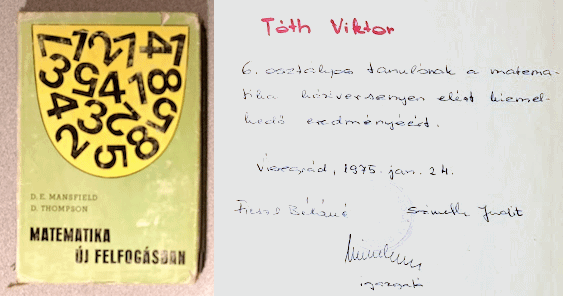
The inscription, written just over 50 years ago, explains that I received this book from my grade school, in recognition for my exceptional results in mathematics as a sixth grade student. (If memory serves me right, this was the year when I unofficially won the Pest county math championship… for eighth graders.)
The book is a Hungarian-language translation of a British volume from the series Mathematics: A New Approach, by D. E. Mansfield and others, published originally in the early 1960s. I passionately loved this book. It was from this book that I first became familiar with many concepts in trigonometry, matrix algebra, and other topics.
Why am I mentioning this volume? Because the other day, the mailman arrived with an Amazon box containing a set of books. A brand new set of books, published in 2024. A series of mathematics textbooks for middle school and high school students, starting with this volume for 6th and 7th graders:
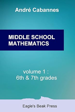
My instant impression: As a young math geek 50 years ago, I would have fallen in love with these books.
The author, André Cabannes, is known, among other things, as Leonard Susskind’s co-author of General Relativity, the latest book in Susskind’s celebrated Theoretical Minimum series. Cabannes also published several books in his native French, along with numerous translations.
His Middle School Mathematics and High School Mathematics books are clearly the works of passion by a talented, knowledgeable, dedicated author. The moment I opened the first volume, I felt a sense of familiarity. I sensed the same clarity, same organization, and the same quality of writing that characterized those Mansfield books all those years ago.
Make no mistake about it, just like the Mansfield books, these books by Cabannes are ambitious. The subjects covered in these volumes go well beyond, I suspect, the mathematics curricula of most middle schools or high schools around the world. So what’s wrong with that, I ask? A talented young student would be delighted, not intimidated, by the wealth of subjects that are covered in the books. The style is sufficiently light-hearted, with relevant illustrations on nearly every page, with the occasional historical tidbit or anecdote, making it easier to absorb the material. And throughout, there is an understanding of the practical nature, utility of mathematics, that is best summarized by the words on the books’ back cover: “Mathematics is not a collection of puzzles or riddles designed to test your intelligence; it is a language for describing and interacting with the world.”
Indeed it is. And these books are true to the author’s words. The subjects may range from the volume of milk cartons through the ratio of ingredients in a cake recipe all the way to the share of the popular vote in the 2024 US presidential election. In each of these examples, the practical utility of numbers and mathematical methods is emphasized. At the same time, the books feel decidedly “old school” but in a good sense: there is no sign of any of the recent fads in mathematics education. The books are “hard core”: ideas and methods are presented in a straightforward way, fulfilling the purpose of passing on the accumulated knowledge of generations to the young reader even as motivations and practical utility are often emphasized.
This is how my love affair with math began when I was a young student, all those years ago. The books that came into my possession, courtesy of both my parents and my teachers, were of a similar nature: they offered robust knowledge, practical utility, clear motivation. Had it existed already, this wonderful series by Cabannes would have made a perfect addition to my little library 50 years ago.
Someone sent me a link to a YouTube podcast, a segment from an interview with a physicist.
I didn’t like the interview. It was about string theory. My dislike is best illustrated by a point that was made by the speaker. He matter-of-factly noted that, well, math is weird, the sum of \(1 + 2 + 3 + …,\) ad infinitum, is \(-\tfrac{1}{12}.\)
This flawlessly illustrates what bothers me both about the state of theoretical physics and about the way it is presented to general audiences.
No, the sum of all positive integers is not \(-\tfrac{1}{12}.\) Not by a longshot. It is divergent. If you insist, you might say that it is infinite. Certainly not a negative rational number.
But where does this nonsense come from?
Well, there’s the famous Riemann zeta-function. For values of \(s>1,\) it is indeed defined as
$$\zeta(s)=\sum_{n=1}^\infty \frac{1}{n^s}.\tag{1}$$
It is a very interesting function, at the heart of some unresolved problems in mathematics.
But the case of \(s=-1\) (which is when the right-hand side of the equation used to define \(\zeta(s)\) corresponds to the sum of all positive integers) is not an unresolved problem. As it is often presented, it is little more than a dirty trick befitting a cheap stage magician, not a scientist.
That is to say, the above definition of \(\zeta(s),\) as I said, is valid only for \(s>1.\) However, the zeta-function has what is called its analytic continuation, which makes it possible to extend the definition for other values of \(s,\) including \(s=-1.\) This can be accomplished utilizing Riemann’s functional equation, \(\zeta(s)=2^s\pi^{s-1}\sin(\tfrac{1}{2}\pi s)\Gamma(1-s)\zeta(1-s).\) But the right-hand side of (1) in this case does not apply! That sum is valid only when it is convergent, which is to say (again), \(s>1.\)
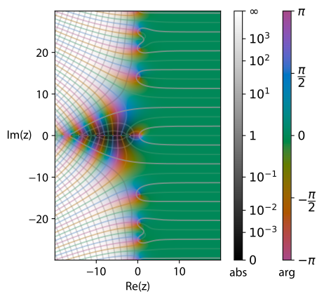
A view of the Riemann zeta-function, from Wikipedia.
So no, the fact that \(\zeta(-1)=-\tfrac{1}{12}\) does not mean that the sum of all integers is \(-\tfrac{1}{12}.\) To suggest otherwise only to dazzle the audience is — looking for a polite term here that nonetheless accurately expresses my disapproval — well, it’s dishonest.
And perhaps unintentionally, it also shows the gap between robust physics and the kind of mathematical games like string theory that pretend to be physics, even though much of it is about mathematical artifacts in 10 dimensions, with at best a very tenuous connection to observable reality.
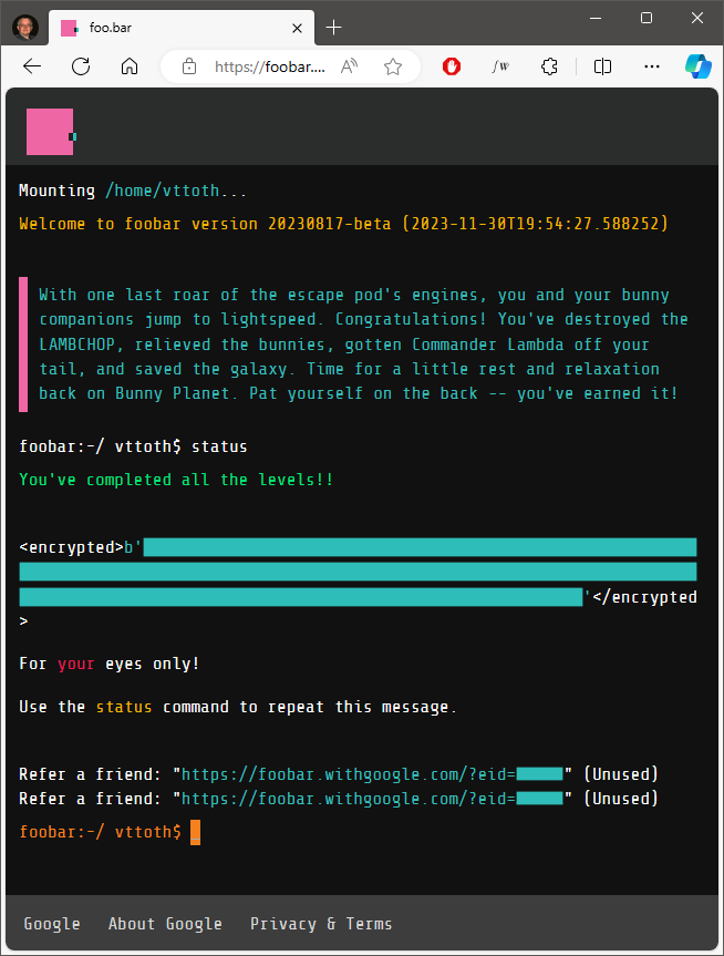
So the other day, as I was doing a Google Search (can’t exactly remember what it was that I was searching for but it was machine learning related), up pops this invitation to participate in a challenge.
Turned out to be the Google Foobar challenge, Google’s secret recruiting tool. (Its existence is not really a secret, so I am not really revealing any great secrets here.)
Though I have no plans to become a Google employee (and I doubt they’re interested in me on account of my age anyway) I decided to go through the challenge because, well, it’s hard to say no to a challenge, and it was an opportunity to practice my Python skills (which need a lot of practice, because I have not yet used Python that much.)
Well, I did it. It was fun.
More importantly, I enjoyed it just as much as I enjoyed similar challenges as a math geek in my early teens. And if that’s not a gift from life, I don’t know what it is.
And yes, I am now much better at Python than I was just a few days ago. I certainly appreciate why the language has become popular, though I can also see its non-trivial pitfalls.
I am simulating gravitational lenses, ray tracing the diffracted light.
With multiple lenses, the results can be absolutely fascinating. Here’s a case of four lenses, three static, a fourth lens transiting in front of the other three, with the light source a fuzzy sphere in the background.
I can’t stop looking at this animation. It almost feels… organic. Yet the math behind it is just high school math, a bit of geometry and trigonometry, nothing more.
NB: This post has been edited with an updated, physically more accurate animation.
I just finished uploading the latest release, 5.47.0, of our beautiful Maxima project.
It was a harder battle than I anticipated, lots of little build issues I had to fix before it was ready to go.
Maxima remains one of the three major computer algebra systems. Perhaps a bit (but only a bit!) less elegant-looking than Mathematica, and perhaps a bit (but only a bit!) less capable on some friends (exotic integrals, differential equations) than Maple, yet significantly more capable on other fronts (especially I believe abstract index tensor algebra and calculus), it also has a unique property: it’s free and open source.
It is also one of the oldest pieces of major software that remains in continuous use. Its roots go back to the 1960s. I occasionally edit 50-year old code in its LISP code base.
And it works. I use it every day. It is “finger memory”, my “go to” calculator, and of course there’s that tensor algebra bit.
Maxima also has a beautiful graphical interface, which I admit I don’t use much though. You might say that I am “old school” given my preference for the text UI, but that’s really not it: the main reason is that once you know what you’re doing, the text UI is simply more efficient.
I hope folks will welcome this latest release.
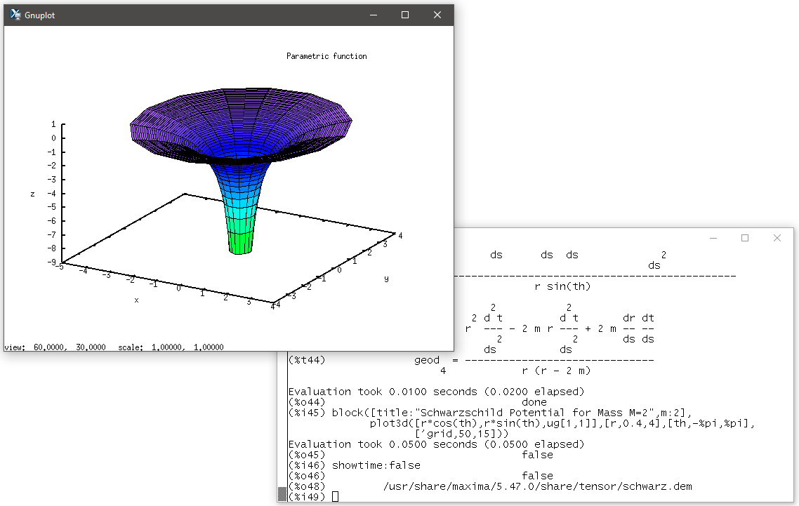
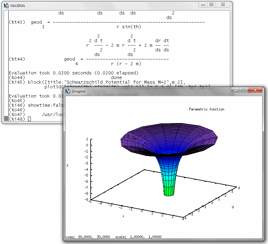
We all know that GPT is very competent, very knowledgeable. So let me go ahead and ask a technical question. It’s not trivial but not terribly complicated either; any student studying general relativity should be able to show the correct derivation. Here is my question:
Derive the geodesic equations for \(d\tau^2=Bdt^2-Adr^2-r^2d\theta^2-r^2\sin^2\theta d\phi^2\), where \(A\) and \(B\) are functions of \(r\) only.
Let’s see how GPT3.5 responds:
The geodesic equations for the given metric are given by:
$$\frac{d^2x^\alpha}{d\tau^2}+\Gamma^\alpha_{\mu\nu}\frac{dx^\mu}{d\tau}\frac{dx^\nu}{d\tau}=0$$
where \(\tau\) is the proper time, \(x^\alpha\) are the coordinates \((t,r,\theta,\phi)\), and \(\Gamma^\alpha_{\mu\nu}\) are the Christoffel symbols of the second kind, given by:
$$\Gamma^\alpha_{\mu\nu}=\frac{1}{2}g^{\alpha\beta}(\partial_\mu g_{\beta\nu}+\partial_\nu g_{\beta\mu}-\partial_\beta g_{\mu\nu})$$
where \(g_{\alpha\beta}\) is the metric tensor.
For the given metric, the non-zero Christoffel symbols are:
\begin{align*}
\Gamma^t_{rr}&=\frac{1}{2}B’\\
\Gamma^t_{tt}&=\frac{1}{2}B\frac{A’}{B}\\
\Gamma^r_{rt}&=\frac{1}{2}\frac{A’}{B}\\
\Gamma^r_{rr}&=-\frac{1}{2}\frac{A’}{B}\\
\Gamma^\theta_{r\theta}&=\frac{1}{r}\\
\Gamma^\theta_{\theta\phi}&=-\sin\theta\cos\theta\\
\Gamma^\phi_{r\phi}&=\frac{1}{r}\\
\Gamma^\phi_{\theta\phi}&=\cot\theta
\end{align*}where a prime denotes differentiation with respect to \(r\).
Using these, we can write down the geodesic equations explicitly:
\begin{align*}
\frac{d^2t}{d\tau^2}+\frac{B’}{2B}\left(\frac{dt}{d\tau}\right)^2+\frac{A’}{2B}\left(\frac{dr}{d\tau}\right)\left(\frac{dt}{d\tau}\right)&=0\\
\frac{d^2r}{d\tau^2}-\frac{A’}{2B}\left(\frac{dt}{d\tau}\right)^2+\frac{A’}{2B}\left(\frac{dr}{d\tau}\right)^2+r\left(\left(\frac{d\theta}{d\tau}\right)^2+\sin^2\theta\left(\frac{d\phi}{d\tau}\right)^2\right)&=0\\
\frac{d^2\theta}{d\tau^2}+2\frac{dr}{d\tau}\frac{d\theta}{d\tau}-\sin\theta\cos\theta\left(\frac{d\phi}{d\tau}\right)^2&=0\\
\frac{d^2\phi}{d\tau^2}+2\frac{dr}{d\tau}\frac{d\phi}{d\tau}+2\cot\theta\frac{d\theta}{d\tau}\frac{d\phi}{d\tau}&=0
\end{align*}
Hmmm… sounds eminently knowledgeable, does it not?
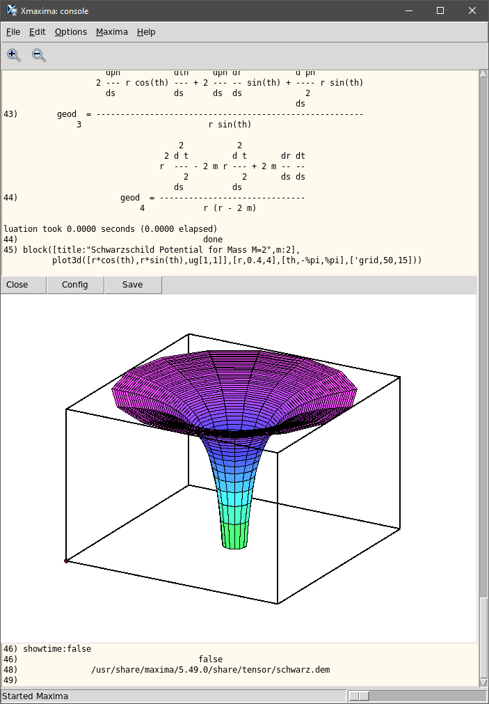
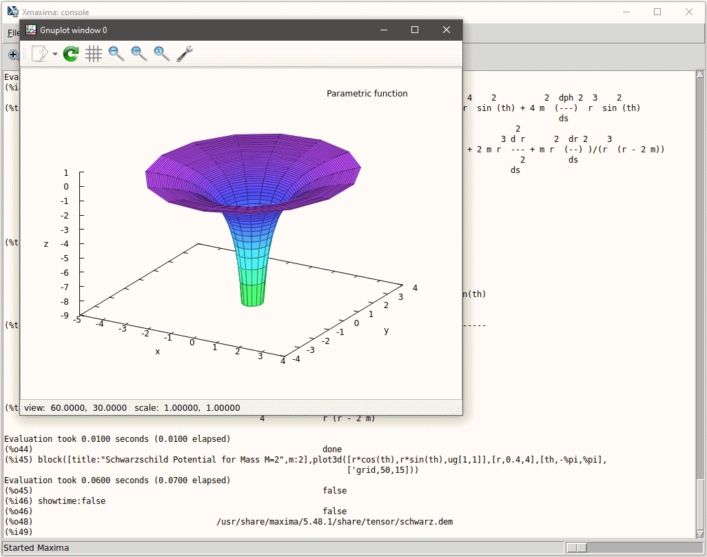
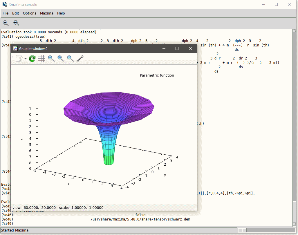
Well… maybe not. How about we ask an actual computer algebra system:
(%i1) load(ctensor)$
(%i2) derivabbrev:true$
(%i3) ct_coords:[t,r,u,v]$
(%i4) depends([A,B],[r])$
(%i5) lg:matrix([B,0,0,0],[0,-A,0,0],[0,0,-r^2,0],[0,0,0,-r^2*sin(u)^2])$
(%i6) cmetric(false)$
(%i7) christof(mcs)$
                                            B
                                             r
(%t7)                          mcs        = ---
                                  1, 1, 2   2 A

                                            B
                                             r
(%t8)                          mcs        = ---
                                  1, 2, 1   2 B

                                            A
                                             r
(%t9)                          mcs        = ---
                                  2, 2, 2   2 A

                                             1
(%t10)                          mcs        = -
                                   2, 3, 3   r

                                             1
(%t11)                          mcs        = -
                                   2, 4, 4   r

                                              r
(%t12)                         mcs        = - -
                                  3, 3, 2     A

                                           cos(u)
(%t13)                        mcs        = ------
                                 3, 4, 4   sin(u)

                                               2
                                          r sin (u)
(%t14)                     mcs        = - ---------
                              4, 4, 2         A

(%t15)                   mcs        = - cos(u) sin(u)
                            4, 4, 3

(%i16) geod:[0,0,0,0]$
(%i17) cgeodesic(true)$
                                   B t    + B  r  t
                                      s s    r  s  s
(%t17)                     geod  = -----------------
                               1           B

                        2        2           2          2                     2
                 2 r sin (u) (v )  + 2 r (u )  - B  (t )  - 2 A r    - A  (r )
                               s           s      r   s          s s    r   s
(%t18) geod  = - --------------------------------------------------------------
           2                                  2 A

                                            2
                        r cos(u) sin(u) (v )  - r u    - 2 r  u
                                          s        s s      s  s
(%t19)        geod  = - ----------------------------------------
                  3                        r

                   r sin(u) v    + 2 r cos(u) u  v  + 2 r  sin(u) v
                             s s               s  s      s         s
(%t20)     geod  = -------------------------------------------------
               4                       r sin(u)
Looks different, doesn’t it. And no, I don’t mean LaTeX vs. the fixed pitch character representations of equations in a text terminal. Rather, the content.
The thing is, what GPT produces looks plausible. It has the right idea. The equations seem to make sense. Unless you know what to expect, you are likely to accept the result as correct, since it appears correct. But GPT sucks at math. It gets easily confused. It is a text model that is optimized to write equations that look right… but only has a superficial understanding of what it produces. Kind of like a student who is trying hard to remember, produces something that resembles the right thing, but without a perfect memory (and keep in mind, trained neural nets are not like any other software we are used to using, as they have no perfect memory!) and without in-depth understanding, fails.
I am sure over time this will improve. GPT-4 is already better at it than 3.5 (which was used to produce this outcome). And future versions may likely interface with computer algebra subsystems (among other things) to augment the neural net with specific capabilities. But for now, perhaps I can be forgiven for asking GPT’s cousin, DALL-E, to draw me a cat, exasperated by the bad math GPT produces:

I’ve been wanting to write about this all the way back in April, when folks became rather upset after Florida rejected some school math textbooks. A variety of reasons were cited, including references to critical race theory and things like social-emotional learning.
Many were aghast: Has the political right gone bonkers, seeing shadows even in math textbooks? And to a significant extent, they were correct: when a textbook is rejected because it uses, as an example, racial statistics in a math problem, or heaven forbid, mentions climate change as established observational fact, you can tell that it’s conservative denialism, not genuine concern about children’s education that is at work.
But was there more to these rejections than ludicrous conservative ideology? Having in the past read essays arguing that mathematics education is “white supremacist”, I certainly could not exclude the possibility. Still, it seemed unlikely. That is, until I came across pages like Mrs. Beattie’s Classroom, explaining “How to spark social-emotional learning in your math classroom“.
Holy freaking macaroni! I thought this nonsense exists only in satire, like a famous past Simpsons episode. But no. These good people think the best way to teach children how to do basic math is through questions like “How did today’s math make you feel?” — “What can you do when you feel stressed out in math class?” — “What self-talk can you use to help you persevere?” or even “How can you be a good group member?” The line between reality and satire does not seem to exist anymore.
In light of this, I cannot exactly blame Florida anymore. Conservatives may be living in a deep state of denial when it comes to certain subjects (way too many of them, from women’s health the climate change) but frankly, this nonsense is almost as freakishly crazy. If I were a parent of a school age child in the United States today, I’d be deeply concerned: Does it really boil down to a choice between schools governed by some form of Christian Taliban or wokeism gone berserk?
From time to time, I promise myself not to respond again to e-mails from strangers, asking me to comment on their research, view their paper, offer thoughts.
Yet from time to time, when the person seems respectable, the research genuine, I do respond. Most of the time, in vain.
Like the other day. Long story short, someone basically proved, as part of a lengthier derivation, that general relativity is always unimodular. This is of course manifestly untrue, but I was wondering where their seemingly reasonable derivation went awry.
Eventually I spotted it. Without getting bogged down in the details, what they did was essentially equivalent to proving that second derivatives do not exist:
$$\frac{d^2f}{dx^2} = \frac{d}{dx}\frac{df}{dx} = \frac{df}{dx}\frac{d}{df}\frac{df}{dx} = \frac{df}{dx}\frac{d}{dx}\frac{df}{df} = \frac{df}{dx}\frac{d1}{dx} = 0.$$
Of course second derivatives do exist, so you might wonder what’s happening here. The sleight of hand happens after the third equal sign: swapping differentiation with respect to two independent variables is permitted, but \(x\) and \(f\) are not independent and therefore, this step is illegal.
I pointed this out, and received a mildly abusive comment in response questioning the quality of my mathematics education. Oh well. Maybe I will learn some wisdom and refrain from responding to strangers in the future.
Came across a question tonight: How do you construct the matrix
$$\begin{pmatrix}1&2&…&n\\n&1&…&n-1\\…\\2&3&…&1\end{pmatrix}?$$
Here’s a bit of Maxima code to make it happen:
(%i1) M(n):=apply(matrix,makelist(makelist(mod(x-k+n,n)+1,x,0,n-1),k,0,n-1))$
(%i2) M(5);
                               [ 1  2  3  4  5 ]
                               [               ]
                               [ 5  1  2  3  4 ]
                               [               ]
(%o2)                          [ 4  5  1  2  3 ]
                               [               ]
                               [ 3  4  5  1  2 ]
                               [               ]
                               [ 2  3  4  5  1 ]
I also ended up wondering about the determinants of these matrices:
(%i3) makelist(determinant(M(i)),i,1,10);
(%o3) [1, - 3, 18, - 160, 1875, - 27216, 470596, - 9437184, 215233605, - 5500000000]
I became curious if this sequence of numbers was known, and indeed that is the case. It is sequence number A052182 in the Encyclopedia of Integer Sequences: “Determinant of n X n matrix whose rows are cyclic permutations of 1..n.” D’oh.
As it turns out, this sequence also has another name: it’s the Smarandache cyclic determinant sequence. In closed form, it is given by
$${\rm SCDNS}(n)=(-1)^{n+1}\frac{n+1}{2}n^{n-1}.$$
(%i4) SCDNS(n):=(-1)^(n+1)*(n+1)/2*n^(n-1);
                                      n + 1
                                 (- 1)      (n + 1)   n - 1
(%o4)               SCDNS(n) := (------------------) n
                                         2
(%i5) makelist(determinant(SCDNS(i)),i,1,10);
(%o5) [1, - 3, 18, - 160, 1875, - 27216, 470596, - 9437184, 215233605, - 5500000000]
Surprisingly, apart from the alternating sign it shares the first several values with another sequence, A212599. But then they deviate.
Don’t let anyone tell you that math is not fun.
Acting as “release manager” for Maxima, the open-source computer algebra system, I am happy to announce that just minutes ago, I released version 5.46.
I am an avid Maxima user myself; I’ve used Maxima’s tensor algebra packages, in particular, extensively in the context of general relativity and modified gravity. I believe Maxima’s tensor algebra capabilities remain top notch, perhaps even unsurpassed. (What other CAS can derive Einstein’s field equations from the Einstein-Hilbert Lagrangian?)
The Maxima system has more than half a century of history: its roots go back to the 1960s, when I was still in kindergarten. I have been contributing to the project for nearly 20 years myself.
Anyhow, Maxima 5.46, here we go! I hope I made no blunders while preparing this release, but if I did, I’m sure I’ll hear about it shortly.
The other day, someone asked a question: Can the itensor package in Maxima calculate the Laplace-Beltrami operator applied to a scalar field in the presence of torsion?
Well, it can. But I was very happy to get this question because it allowed me to uncover some long-standing, subtle bugs in the package that prevented some essential simplifications and in some cases, even produced nonsensical results.
With these fixes, Maxima now produces a beautiful result, as evidenced by this nice newly created demo, which I am about to add to the package:
(%i1) if get('itensor,'version) = false then load(itensor)
(%i2) "First, we set up the basic properties of the system"
(%i3) imetric(g)
(%i4) "Demo is faster in 3D but works for other values of dim, too"
(%i5) dim:3
(%i6) "We declare symmetries of the metric and other symbols"
(%i7) decsym(g,2,0,[sym(all)],[])
(%i8) decsym(g,0,2,[],[sym(all)])
(%i9) components(g([a],[b]),kdelta([a],[b]))
(%i10) decsym(levi_civita,0,dim,[],[anti(all)])
(%i11) decsym(itr,2,1,[anti(all)],[])
(%i12) "It is useful to set icounter to avoid indexing conflicts"
(%i13) icounter:100
(%i14) "We choose the appropriate convention for exterior algebra"
(%i15) igeowedge_flag:true
(%i16) "Now let us calculate the Laplacian of a scalar field and simplify"
(%i17) canform(hodge(extdiff(hodge(extdiff(f([],[]))))))
(%i18) contract(expand(lc2kdt(%)))
(%i19) ev(%,kdelta)
(%i20) D1:ishow(canform(%))
                  %1 %2  %3 %4                 %1 %2            %1 %2
(%t20)   (- f    g      g      g     ) + f    g      + f       g
             ,%4  ,%3           %1 %2     ,%2  ,%1      ,%1 %2
(%i21) "We can re-express the result using Christoffel symbols, too"
(%i22) ishow(canform(conmetderiv(D1,g)))
               %1 %4  %2 %5      %3                   %1 %2      %3
(%t22) 2 f    g      g      ichr2      g      - f    g      ichr2
          ,%5                    %1 %2  %3 %4    ,%3             %1 %2
                                              %1 %3      %2               %1 %2
                                      - f    g      ichr2      + f       g
                                         ,%3             %1 %2    ,%1 %2
(%i23) "Nice. Now let us repeat the same calculation with torsion"
(%i24) itorsion_flag:true
(%i25) canform(hodge(extdiff(hodge(extdiff(f([],[]))))))
(%i26) "Additional simplifications are now needed"
(%i27) contract(expand(lc2kdt(%th(2))))
(%i28) ev(%,kdelta)
(%i29) canform(%)
(%i30) ev(%,ichr2)
(%i31) ev(%,ikt2)
(%i32) ev(%,ikt1)
(%i33) ev(%,g)
(%i34) ev(%,ichr1)
(%i35) contract(rename(expand(canform(%))))
(%i36) flipflag:not flipflag
(%i37) D2:ishow(canform(%th(2)))
                %1 %2  %3 %4                 %1 %2    %3            %1 %2
(%t37) (- f    g      g      g     ) + f    g      itr      + f    g
           ,%1         ,%2    %3 %4     ,%1           %2 %3    ,%1  ,%2
                                                                          %1 %2
                                                               + f       g
                                                                  ,%1 %2
(%i38) "Another clean result; can also be expressed using Christoffel symbols"
(%i39) ishow(canform(conmetderiv(D2,g)))
               %1 %2  %3 %4      %5                   %1 %2    %3
(%t39) 2 f    g      g      ichr2      g      + f    g      itr
          ,%1                    %2 %3  %4 %5    ,%1           %2 %3
                     %1 %2      %3            %2 %3      %1               %1 %2
             - f    g      ichr2      - f    g      ichr2      + f       g
                ,%1             %2 %3    ,%1             %2 %3    ,%1 %2
(%i40) "Finally, we see that the two results differ only by torsion"
(%i41) ishow(canform(D2-D1))
                                   %1 %2    %3
(%t41)                       f    g      itr
                              ,%1           %2 %3
(%i42) "Last but not least, d^2 is not nilpotent in the presence of torsion"
(%i43) extdiff(extdiff(f([],[])))
(%i44) ev(%,icc2,ikt2,ikt1)
(%i45) canform(%)
(%i46) ev(%,g)
(%i47) ishow(contract(%))
                                       %3
(%t47)                         f    itr
                                ,%3    %275 %277
(%i48) "Reminder: when dim = 2n, the Laplacian is -1 times these results."
The learning curve is steep and there are many pitfalls, but itensor remains an immensely powerful package.
We just released another beautiful new version of Maxima, 5.45.0. This time around, it also includes changes (for the first time in years) to the tensor packages, based on a very comprehensive set of proposed patches by a devoted Maxima user.
A popular Internet meme these days is to present an arithmetic expression like, say, 6/3(4−2) and ask the poor souls who follow you to decide the right answer. Soon there will be two camps, each convinced that they know the truth and that the others are illiterate fools: According to one camp, the answer is 4, whereas the other camp will swear that it has to be 1.
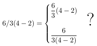
In reality it is neither. Or both. Flip a coin, take your pick. There is no fundamental mathematical truth hidden here. It all boils down to human conventions. The standard convention is that multiplication and division have the same precedence and are evaluated from left to right: So 6/3×(4−2) is pretty unambiguous. But there is another, unwritten convention that when the multiplication sign is omitted, the implied multiplication is assumed to have a higher precedence.
Precisely because of these ambiguities, when you see actual professionals, mathematicians or physicists, write down an expression like this, they opt for clarity: they write, say, (6/3)(4−2) or 6/[3(4−2)] precisely so as to avoid any misunderstanding. Or better yet, they use proper math typesetting software such as LaTeX and write 2D formulas.
 I met Gabor David back in 1982 when I became a member of the team we informally named F451 (inspired by Ray Bradbury of course.) Gabor was a close friend of Ferenc Szatmari. Together, they played an instrumental role in establishing a business relationship between the Hungarian firm Novotrade and its British partner, Andromeda, developing game programs for the Commodore 64.
In the months and years that followed, we spent a lot of time working together. I was proud to enjoy Gabor’s friendship. He was very knowledgeable, and also very committed to our success. We had some stressful times, to be sure, but also a lot of fun, frantic days (and many nights!) spent working together.
I remember Gabor’s deep, loud voice, with a slight speech impediment, a mild case of rhotacism. His face, too, I can recall with almost movie like quality.
He loved coffee more than I thought possible. He once dropped by at my place, not long after I managed to destroy my coffee maker, a stovetop espresso that I accidentally left on the stove for a good half hour. Gabor entered with the words, “Kids, do you have any coffee?” I tried to explain to him that the devil’s brew in that carafe was a bitter, undrinkable (and likely unhealthy) blend of burnt coffee and burnt rubber, but to no avail: he gulped it down like it was nectar.
After I left Hungary in 1986, we remained in sporadic contact. In fact, Gabor helped me with a small loan during my initial few weeks on Austria; for this, I was very grateful.
When I first visited Hungary as a newly minted Canadian citizen, after the collapse of communism there, Gabor was one of the few close friends that I sought out. I was hugely impressed. Gabor was now heading a company called Banknet, an international joint venture bringing business grade satellite-based Internet service to the country.
When our friend Ferenc was diagnosed with lung cancer, Gabor was distraught. He tried to help Feri with financing an unconventional treatment not covered by insurance. I pitched in, too. It was not enough to save Feri’s life: he passed away shortly thereafter, a loss I still feel more than two decades later.
My last conversation with Gabor was distressing. I don’t really remember the details, but I did learn that he suffered a stroke, and that he was worried that he would be placed under some form of guardianship. Soon thereafter, I lost touch; his phone number, as I recall, was disconnected and Gabor vanished.
Every so often, I looked for him on the Internet, on social media, but to no avail. His name is not uncommon, and moreover, as his last name also doubles as a first name for many, searches bring up far too many false positives. But last night, it occurred to me to search for his name and his original profession: “Dávid Gábor” “matematikus” (mathematician).
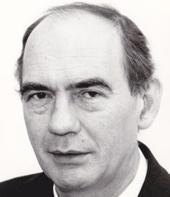
Jackpot, if it can be called that. One of the first hits that came up was a page from Hungary’s John von Neumann Computer Society, their information technology history forum, to be specific: a short biography of Gabor, together with his picture.
And from this page I learned that Gabor passed away almost six years ago, on November 10, 2014, at the age of 72.
Well… at least I now know. It has been a privilege knowing you, Gabor, and being able to count you among my friends. I learned a lot from you, and I cherish all those times that we spent working together.
Long overdue, but I just finished preparing the latest Maxima release, version 5.44.
I am always nervous when I do this. It is one thing to mess with my own projects, it is another thing to mess with a project that is the work of many people and contains code all the way back from the 1960s.
I am one of the maintainers of the Maxima computer algebra system. Maxima’s origins date back to the 1960s, when I was still in kindergarten. I feel very privileged that I can participate in the continuing development of one of the oldest continuously maintained software system in wide use.
It has been a while since I last dug deep into the core of the Maxima system. My LISP skills are admittedly a bit rusty. But a recent change to a core Maxima capability, its ability to create Taylor-series expansions of expressions, broke an important feature of Maxima’s tensor algebra packages, so it needed fixing.
The fix doesn’t amount to much, just a few lines of code:
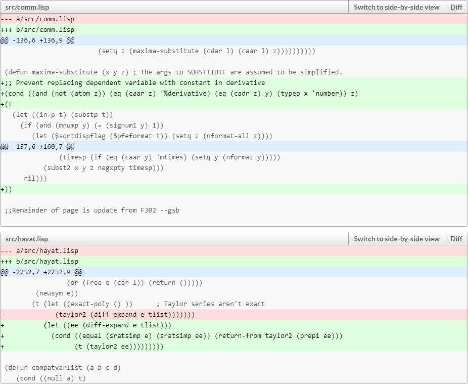
It did take more than a few minutes though to find the right (I hope) way to implement this fix.
Even so, I had fun. This is the kind of programming that I really, really enjoy doing. Sadly, it’s not the kind of programming for which people usually pay you Big Bucks… Oh well. The fun alone was worth it.