May 2020 – Spinor Info

The more maps, the merrier

May 242020

Still playing with some COVID-19 maps, so here is another one: This one ranks countries by the number of COVID-19 cases per 1,000 square kilometers.

What’s the point, you might ask? Well, when there are lots of people confined to a small area, even a few cases can mean trouble; in contrast, when you have many cases but spread over half a continent, you may never come across a single infected person in your travels.

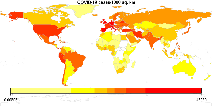
Again, the color legend remains a little whacky; it is logarithmic, but I don’t know how to convince this R package to display it nicely.

The numbers are pretty high. It goes without saying that densely populated microstates like Monaco win the contest, but then there is Qatar (3494), Belgium (1866), the Netherlands (1324), the UK (1051)… numbers that are way too high. For comparison, the USA is at 180, Hungary at 41, Russia at 20 (no surprise there), China at 9 (!), and so is Canada.

A more encouraging plot

Health No Responses »

May 232020

Maps that show the spread and mortality rate of COVID-19 are worrisome, to say the least.

So here is something slightly more encouraging: the day-to-day growth rate of COVID-19 infections, in the world, the United States, Canada, and the province of Ontario where I live.

What this plot shows is that the growth rate has been consistently and steadily decreasing (note that the vertical axis is logarithmic). Furthermore, the overall behavior of the worldwide, US, and Canadian plots is remarkable similar.

Of course this plot is also a reflection of the fact that the cumulative number of cases increases, so even if the number of new cases remains steady, the growth rate will indeed decrease. Nonetheless, it demonstrates that at least for now, the pandemic’s exponential spread has been arrested. This can, of course, change for the worse quite dramatically if we lose our collective patience and start relaxing too soon.

Some COVID-19 maps

Health No Responses »

May 232020

I suppose the most important thing to know about COVID-19 is not so much the total number of cases or deaths, but the number of cases or deaths per million people. A number like 1,000 deaths is huge in a country of one million, a drop in the bucket in a country like India or China.

In that vein, I produced two maps using my rather rusty R programming skills. I am sure I could have done a better job labeling the legend, but there is only so much time I wanted to spend on this. The color bar legend is logarithmic between its two end values.

First, the cumulative number of cases per million people (May 22 data):

Next, deaths per million:

Not a pretty picture. It appears that the countries that are the most disproportionately affected (or the most likely to offer accurate reports?) are in Europe (including Russia), North and South America and the Middle East.

But now, here is perhaps the scariest map of all:

Yes, in many countries more than 10% of the confirmed cases result in death. The global average is 6.4 per 100 confirmed cases. The fact that COVID-19 is deadly in countries with underdeveloped health care systems is perhaps understandable, but the fact that the reddest parts of the map are places with the most sophisticated health care systems in the world is food for thought.

Wearing my LISP hat

Computer Algebra, Personal, Programming No Responses »

May 222020

I am one of the maintainers of the Maxima computer algebra system. Maxima’s origins date back to the 1960s, when I was still in kindergarten. I feel very privileged that I can participate in the continuing development of one of the oldest continuously maintained software system in wide use.

It has been a while since I last dug deep into the core of the Maxima system. My LISP skills are admittedly a bit rusty. But a recent change to a core Maxima capability, its ability to create Taylor-series expansions of expressions, broke an important feature of Maxima’s tensor algebra packages, so it needed fixing.

The fix doesn’t amount to much, just a few lines of code:

It did take more than a few minutes though to find the right (I hope) way to implement this fix.

Even so, I had fun. This is the kind of programming that I really, really enjoy doing. Sadly, it’s not the kind of programming for which people usually pay you Big Bucks… Oh well. The fun alone was worth it.

The Shadow of the Black Hole

Books, Personal, Physics No Responses »

May 192020

One of the most fortunate moments in my life occurred in the fall of 2005, when I first bumped into John Moffat, a physicist from The Perimeter Institute in Waterloo, Ontario, Canada, when we both attended the first Pioneer Anomaly conference hosted by the International Space Science Institute in Bern, Switzerland.

This chance encounter turned into a 15-year collaboration and friendship. It was, to me, immensely beneficial: I learned a lot from John who, in his long professional career, has met nearly every one of the giants of 20th century physics, even as he made his own considerable contributions to diverse areas ranging from particle physics to gravitation.

In the past decade, John also wrote a few books for a general audience. His latest, The Shadow of the Black Hole, is about to be published; it can already be preordered on Amazon. In their reviews, Greg Landsberg (CERN), Michael Landry (LIGO Hanford) and Neil Cornish (eXtreme Gravity Institute) praise the book. As I was one of John’s early proofreaders, I figured I’ll add my own.

John began working on this manuscript shortly after the announcement by the LIGO project of the first unambiguous direct detection of gravitational waves from a distant cosmic event. This was a momentous discovery, opening a new chapter in the history of astronomy, while at the same time confirming a fundamental prediction of Einstein’s general relativity. Meanwhile, the physics world was waiting with bated breath for another result: the Event Horizon Telescope collaboration’s attempt to image, using a worldwide network of radio telescopes, either the supermassive black hole near the center of our own Milky Way, or the much larger supermassive black hole near the center of the nearby galaxy M87.

Bookended by these two historic discoveries, John’s narrative invites the reader on a journey to understand the nature of black holes, these most enigmatic objects in our universe. The adventure begins in 1784, when the Reverend John Michell, a Cambridge professor, speculated about stars so massive and compact that even light would not be able to escape from its surface. The story progresses to the 20th century, the prediction of black holes by general relativity, and the strange, often counterintuitive results that arise when our knowledge of thermodynamics and quantum physics is applied to these objects. After a brief detour into the realm of science-fiction, John’s account returns to the hard reality of observational science, as he explains how gravitational waves can be detected and how they fit into both the standard theory of gravitation and its proposed extensions or modifications. Finally, John moves on to discuss how the Event Horizon Telescope works and how it was able to create, for the very first time, an actual image of the black hole’s shadow, cast against the “light” (radio waves) from its accretion disk.

John’s writing is entertaining, informative, and a delight to follow as he accompanies the reader on this fantastic journey. True, I am not an unbiased critic. But don’t just take my word for it; read those reviews I mentioned at the beginning of this post, by preeminent physicists. In any case, I wholeheartedly recommend The Shadow of the Black Hole, along with John’s earlier books, to anyone with an interest in physics, especially the physics of black holes.

Time to get technical (a little cosmology)

Physics No Responses »

May 112020

Heaven knows why I sometimes get confused by the simplest things.

In this case, the conversion between two commonly used cosmological coordinate systems: Comoving coordinates vs. coordinates that are, well, not comoving, in which cosmic expansion is ascribed to time dilation effects instead.

In the standard coordinates that are used to describe the homogeneous, isotropic universe of the Friedmann–Lemaître–Robertson–Walker (FLRW) metric, the metric is given by

$$ds^2=dt^2-a^2dR^2,$$

where $a=a(t)$ is a function of the time coordinate, and $R$ represents the triplet of spatial coordinates: e.g., $dR^2=dx^2+dy^2+dz^2.$

I want to transform this using $R’=aR,$ i.e., transform away the time-dependent coefficient in front of the spatial term in the metric. The confusion comes because for some reason, I always manage to convince myself that I also have to make the simultaneous replacement $t’=a^{-1}dt.$

I do not. This is nonsense. I just need to introduce $dR’$. The rest then presents itself automatically:

$$\begin{align*}
R’&=aR,\\
dR&=d(a^{-1}R’)=-a^{-2}\dot{a}R’dt+a^{-1}dR’,\\
ds^2&=dt^2-a^2[-a^{-2}\dot{a}R’dt+a^{-1}dR’]^2\\
&=(1-a^{-2}\dot{a}^2{R’}^2)dt^2+2a^{-1}\dot{a}R’dtdR’-d{R’}^2\\
&=(1-H^2{R’}^2)dt^2+2HR’dtdR’-d{R’}^2,
\end{align*}$$

where $H=\dot{a}/a$ as usual.

OK, now that I recorded this here in my blog for posterity, perhaps the next time I need it, I’ll remember where to find it. For instance, the next time I manage to stumble upon one of my old Quora answers that, for five and a half years, advertised my stupidity to the world by presenting an incorrect answer on this topic.

This, incidentally, would serve as a suitable coordinate system representing the reference frame of an observer at the origin. It also demonstrates that such an observer sees an apparent horizon, the cosmological horizon, given by $1-H^2{R’}^2=0,$, i.e., $R’=H^{-1},$ the distance characterized by the inverse of the Hubble parameter.

Some probability distributions

Mathematics No Responses »

May 052020

So here I am, reading about some trivial yet not-so-trivial probability distributions.

Let’s start with the uniform distribution. Easy-peasy, isn’t it: a random number, between 0 and 1, with an equal probability assigned to any value within this range.

So… what happens if I take two such random numbers and add them? Why, I get a random number between 0 and 2 of course. But the probability distribution will no longer be uniform. There are more ways to get a value in the vicinity of 1 than near 0 or 2.

And what happens if I add three such random numbers? Or four? And so on?

The statistics of this result are captured by the Irwin-Hall distribution, defined as

$$f_{\rm IH}(x,n)=\dfrac{1}{2(n-1)!}\sum\limits_{k=1}^n(-1)^k\begin{pmatrix}n\\k\end{pmatrix}(x-k)^{n-1}{\rm sgn}(x-k).$$

OK, so that’s what happens when we add these uniformly generated random values. What happens when we average them? This, in turn, is captured by the Bates distribution, which, unsurprisingly, is just the Irwin-Hall distribution, scaled by the factor $n$:

$$f_{\rm B}(x,n)=\dfrac{n}{2(n-1)!}\sum\limits_{k=1}^n(-1)^k\begin{pmatrix}n\\k\end{pmatrix}(nx-k)^{n-1}{\rm sgn}(nx-k).$$

How about that.

For what it’s worth, here is the Maxima script to generate the Irwin-Hall plot:

fI(x,n):=1/2/(n-1)!*sum((-1)^k*n!/k!/(n-k)!*(x-k)^(n-1)*signum(x-k),k,0,n);
plot2d([fI(x,1),fI(x,2),fI(x,4),fI(x,8),fI(x,16)],[x,-2,18],[box,false],
       [legend,"n=1","n=2","n=4","n=8","n=16"],[y,-0.1,1.1]);

And this one for the Bates plot:

fB(x,n):=n/2/(n-1)!*sum((-1)^k*n!/k!/(n-k)!*(n*x-k)^(n-1)*signum(n*x-k),k,0,n);
plot2d([fB(x,1),fB(x,2),fB(x,4),fB(x,8),fB(x,16)],[x,-0.1,1.1],[box,false],
       [legend,"n=1","n=2","n=4","n=8","n=16"],[y,-0.1,5.9]);

Yes, I am still a little bit of a math geek at heart.

Number theory, petals and necklaces

Mathematics, Personal No Responses »

May 022020

My lovely wife, Ildiko, woke up from a dream and asked: If you have a flower with 7 petals and two colors, how many ways can you color the petals of that flower?

Intriguing, isn’t it.

Such a flower shape obviously has rotational symmetry. Just because the flower is rotated by several times a seventh of a revolution, the resulting pattern should not be counted as distinct. So it is not simply calculating what number theorists call the $n$-tuple. It is something more subtle.

We can, of course, start counting the possibilities the brute force way. It’s not that difficult for a smaller number of petals, but it does get a little confusing at 6. At 7 petals, it is still something that can be done, but the use of paper-and-pencil is strongly recommended.

So what about the more general case? What if I have $n$ petals and $k$ colors?

Neither of us could easily deduce an answer, so I went to search the available online literature. For a while, other than finding some interesting posts about cyclic, or circular permutations, I was mostly unsuccessful. In fact, I began to wonder if this one was perhaps one of those embarrassing little problems in combinatorial mathematics that has no known solution and about which the literature remains strangely quiet.

But then I had another idea: By this time, we both calculated the sequence, 2, 3, 4, 6, 8, 14, 20, which is the number of ways flowers with 1, 2, …, 7 petals can be colored using only two colors. Surely, this sequence is known to Google?

Indeed it is. It turns out to be a well-known sequence in the online encyclopedia of integer sequences, A000031. Now I was getting somewhere! What was especially helpful is that the encyclopedia mentioned necklaces. So that’s what this problem set is called! Finding the Mathworld page on necklaces was now easy, along with the corresponding Wikipedia page. I also found an attempt, valiant though only half-successful if anyone is interested in my opinion, to explain the intuition behind this known result:

$$N_k(n)=\frac{1}{n}\sum_{d|n}\phi(d)k^{n/d},$$

where the summation is over all the divisors of $n$, and $\phi(d)$ is Euler’s totient function, the number of integers between $1$ and $d$ that are relative prime to $d$.

Evil stuff if you asked me. Much as I always liked mathematics, number theory was not my favorite.

In the case of odd primes, such as the number 7 that occurred in Ildiko’s dream, and only two colors, there is, however, a simplified form:

$$N_2(n)=\frac{2^{n-1}-1}{n}+2^{(n-1)/2}+1.$$

Unfortunately, this form is for “free necklaces”, which treats mirror images as equivalent. For $n<6$ it makes no difference, but substituting $n=7$, we get 18, not 20.

Finally, a closely related sequence, A000029, characterizes necklaces that can be turned over, that is to say, the case where we do not count mirror images separately.

Oh, this was fun. It’s not like I didn’t have anything useful to do with my time, but it was nonetheless a delightful distraction. And a good thing to chat about while we were eating a wonderful lunch that Ildiko prepared today.