I have been reading a lot today about the latest news from Europe, the supposed confirmation that the elementary particle observed at CERN may indeed by the Higgs boson.
And while they are probably right, I feel that the strong pronouncements may be a little premature and perhaps unwarranted.
Let me demonstrate my thoughts using a simple example and some pretty pictures.
Suppose you go to a camp site. At that camp site there are five buildings, each of the buildings housing a different team. One may be a literary club, another may be a club of chess enthusiasts… but you have reason to believe that one of the buildings is actually occupied by the Harlem Globetrotters.
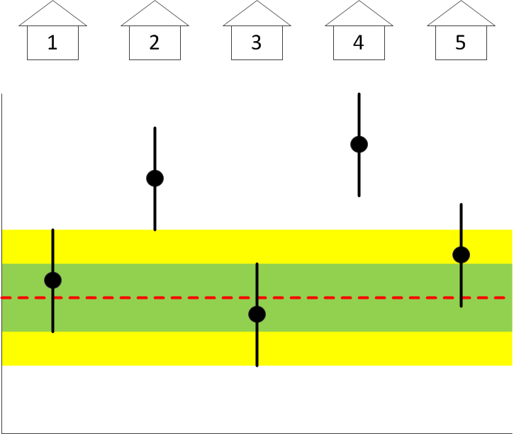
Suppose that the only measurement available to you is a measurement of the average height of the people housed in each of the buildings. You of course know what the mean height and its standard deviation are for the entire population. So then, suppose you are presented with a graph that shows the average height, with error bars, of the people housed in each of five buildings:
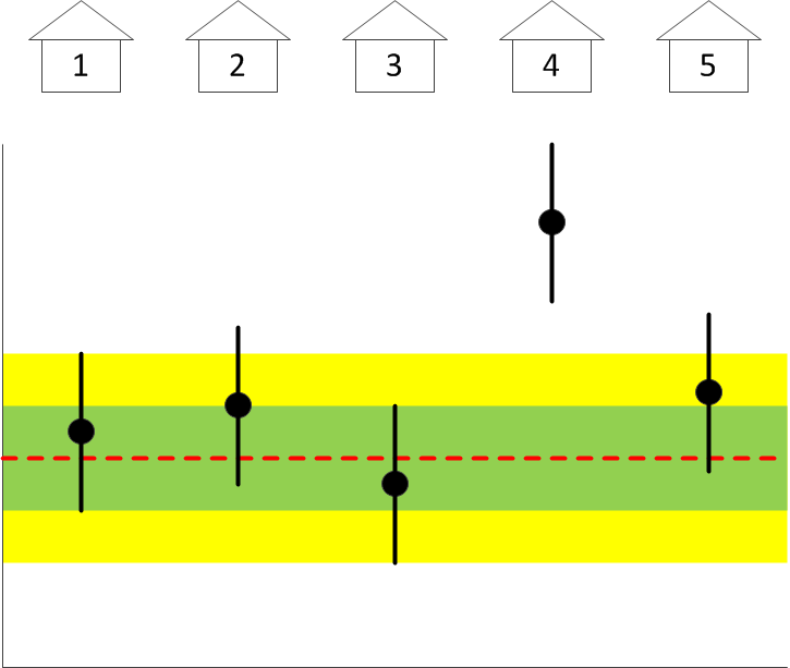
The red dashed line is the population average; the green and yellow shaded areas correspond to one and two standard deviations; and the black dots are the actual data points, with standard deviations, representing the average height of the residents in each of the five buildings.
Can you confirm from this diagram that one of the buildings may indeed be housing the Harlem Globetrotters? Can you guess which one? Why, it’s #4. Easy, wasn’t it. It is the only building in which the average height of the residents deviates from the population (background) average significantly, whereas the heights of the residents of all the other buildings are consistent with the “null hypothesis”, namely that they are random people from the population background.
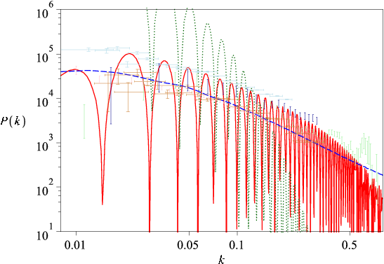
But suppose instead that the graph looks like this:
Can you still tell which building houses the Globetrotters? Guess not. It could be #2… or it could be #4. But if you have other reasons to believe that #4 houses the Globetrotters, you can certainly use this data set as a means of confirmation, even though you are left wondering why #2 also appears perhaps as an outlier. But then, outliers sometimes happen as mere statistical flukes.
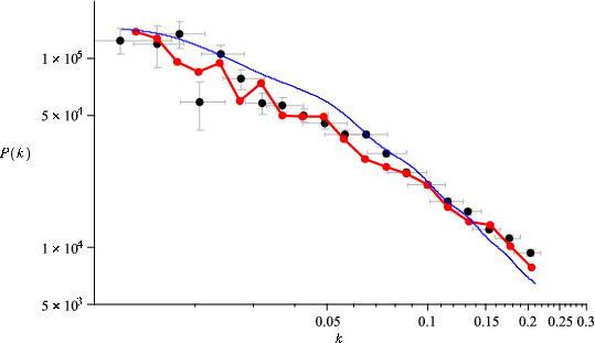
But suppose instead that you see a plot like this one:
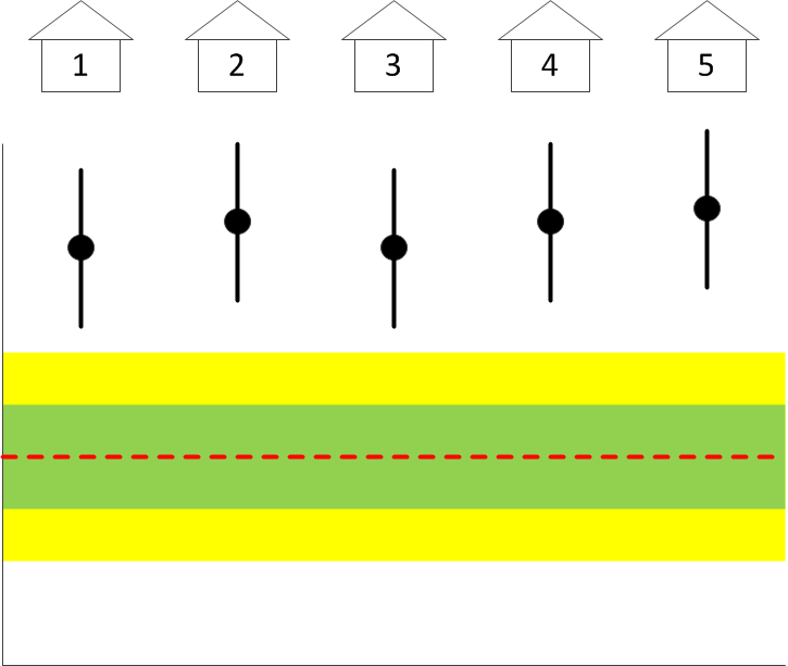
What can you conclude from this plot? Can you conclude anything? Is this a real measurement result and perhaps the entire camp site has been taken over by tall basketball players? Or perhaps you have a systematic error in your measurement, using the wrong ruler maybe? You simply cannot tell. More importantly, you absolutely cannot tell whether or not any of the buildings houses the Harlem Globetrotters, much less which one. Despite the fact that building #4 is still about four standard deviations away from the population average. Until you resolve the issue of the systematic, this data set cannot be used to conclude anything.
But then, why are we told that a similar-looking plot, this one indicating the rate of Higgs boson decay into a pair of τ particles (the heaviest cousin of the electron), indicates a “local significance of 2.9σ”? With a “best fit μ = 1.1 ± 0.4” for a 125 GeV Higgs boson?
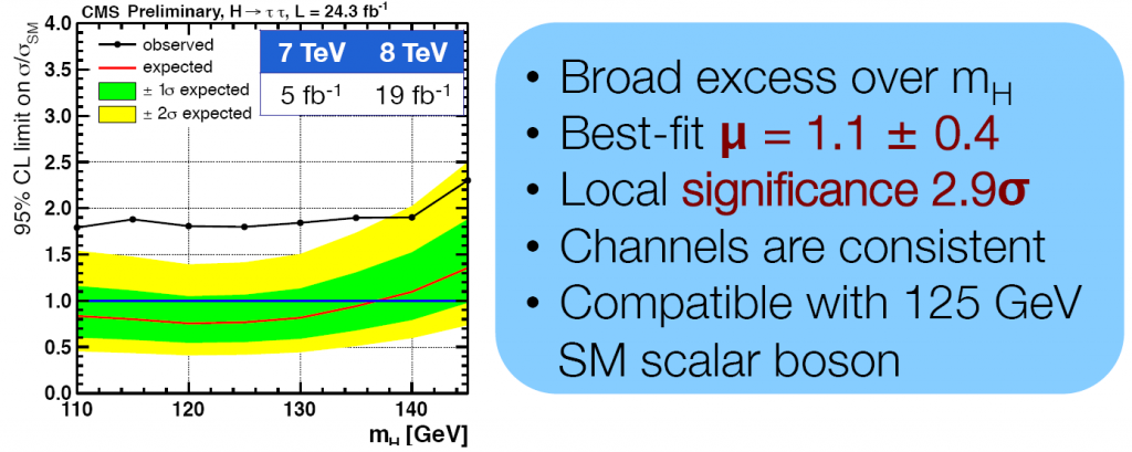
It indicates no such thing. The only thing this plot actually indicates is the presence of an unexplained systematic bias.
Or am I being stubbornly stupid here?
 To the esteemed dinosaurs in charge of whatever our timekeeping bureaucracies happen to be: stop this nonsense already. We no more need daylight savings time in 2013 than we need coal rationing.

 Chances are that if you tuned your television to a news channel these past couple of days, it was news from the skies that filled the screen. First, it was about asteroid 2012DA14, which flew by the planet at a relatively safe distance of some 28,000 kilometers. But even before this asteroid reached its point of closest approach, there was the striking and alarming news from the Russian city of Chelyabinsk: widespread damage and about a thousand people injured as a result of a meteor that exploded in the atmosphere above the city.
 I always thought of myself as a moderate conservative. I remain instinctively suspicious of liberal activism, and I do support some traditionally conservative ideas such as smaller governments, lower taxes, or individual responsibility.
 John Marburger had an unenviable role as Director of the United States Office of Science and Technology Policy. Even before he began his tenure, he already faced demotion: President George W. Bush decided not to confer upon him the title “Assistant to the President on Science and Technology”, a title born both by his predecessors and also his successor. Marburger was also widely criticized by his colleagues for his efforts to defend the Bush Administration’s scientific policies. He was not infrequently labeled a “prostitute” or worse.

 A few weeks ago, I exchanged a number of e-mails with someone about the Lanczos tensor and the Weyl-Lanczos equation. One of the things I derived is worth recording here for posterity.