I have received a surprising number of comments to my recent post on the gravitational potential, including a criticism: namely that what I am saying is nonsense, that in fact it is well known (there is actually a resolution by the International Astronomical Union to this effect) that in the vicinity of the Earth, the gravitational potential is well approximated using the Earth’s multipole plus tidal contributions, and that the potential, therefore, is determined primarily by the Earth itself, the Sun only playing a minor role, contrary to what I was blabbering about.
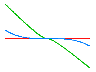
But this is precisely the view of gravity that I was arguing against. As they say, a picture is worth a thousand words, so let me try to demonstrate it with pictures, starting with this one:
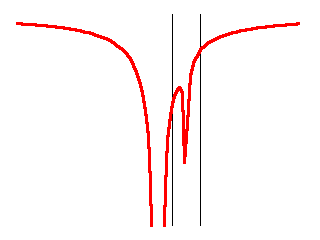
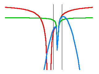
It is a crude one-dimensional depiction of the Earth’s gravity well (between the two vertical black lines) embedded in the much deeper gravity well (centered) of the Sun. In other words, what I depicted is the sum of two gravitational potentials:
$$U=-\frac{GM}{R}-\frac{Gm}{r}.$$
Let me now zoom into the area marked by the vertical lines for a better view:
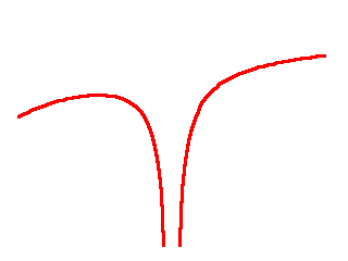
It looks like a perfectly ordinary gravitational potential well, except that it is slightly lopsided.
So what if I ignored the Sun’s potential altogether? In other words, what if I considered the potential given by
$$U=-\frac{Gm}{r}+C$$
instead, where \(C\) is just some normalization constant to ensure that I am comparing apples to apples here? This is what I get:
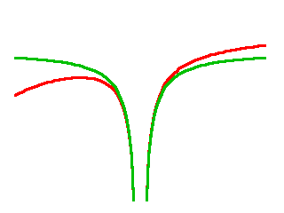
The green curve approximates the red curve fairly well deep inside the potential well but fails further out.
But wait a cotton-picking minute. When I say “approximate”, what does that tell you? Why, we approximate curves with Taylor series, don’t we, at least when we can. The Sun’s gravitational potential, \(-GM/R\), near the vicinity of the Earth located at \(R=R_0\), would be given by the approximation
$$-\frac{GM}{R}=-\frac{GM}{R_0}+\frac{GM}{R_0^2}(R-R_0)-\frac{GM}{R_0^3}(R-R_0)^2+{\cal O}\left(\frac{GM}{R_0^4}[R-R_0]^3\right).$$
And in this oversimplified one-dimensional case, \(r=R-R_0\) so I might as well write
$$-\frac{GM}{R}=-\frac{GM}{R_0}+\frac{GM}{R_0^2}r-\frac{GM}{R_0^3}r^2+{\cal O}\left(\frac{GM}{R_0^4}r^3\right).$$
(In the three-dimensional case, the math gets messier but the principle remains the same.)
So when I used a constant previously, its value would have been \(C=-GM/R_0\) and this would be just the zeroeth order term in the Taylor series expansion of the Sun’s potential. What if I include more terms and write:
$$U\simeq-\frac{Gm}{r}-\frac{GM}{R_0}+\frac{GM}{R_0^2}r-\frac{GM}{R_0^3}r^2?$$
When I plot this, here is what I get:
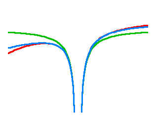
The blue curve now does a much better job approximating the red one. (Incidentally, note that if I differentiate by \(r\) to obtain the acceleration, I get: \(a=-dU/dr=-Gm/r^2-GM/R_0^2+2GMr/R_0^3\), which is the sum of the terrestrial acceleration, the solar acceleration that determines the Earth’s orbit around the Sun, and the usual tidal term. So this is another way to derive the tidal term. But, I digress.)
The improvement can also be seen if I plot the relative error of the green vs. blue curves:
So far so good. But the blue curve still fails miserably further outside. Let me zoom back out to the scale of the original plot:
Oops.
So while it is true that in the vicinity of the Earth, the tidal potential is a useful approximation, it is not the “real thing”. And when we perform a physical experiment that involves, e.g., a distant spacecraft or astronomical objects, the tidal potential must not be used. Such experiments, for instance tests measuring gravitational time dilation or the gravitational frequency shift of an electromagnetic signal are readily realizable nowadays with precision equipment.
But it just occurred to me that even at the pure Newtonian level, the value of the potential \(U\) plays an observable role: it determines the escape velocity. A projectile escapes to infinity if its overall energy (kinetic plus potential) is greater than zero: \(mv^2/2 + mU>0\). In other words, the escape velocity \(v\) is determined by the formula
$$v>\sqrt{-2U}.$$
The escape velocity works both ways; it also tells you the velocity to which an object accelerates as it falls from infinity. So suppose you let lose a rock somewhere in deep space far from the Sun and it falls towards the Earth. Its velocity at impact will be 43.6 km/s… without the Sun’s influence, its impact velocity would have been only 11.2 km/s.
So using somewhat more poetic language, the relationship of us, surface dwellers, to distant parts of the universe, is determined primarily not by the gravity of the planet on which we stand, but by the gravitational field of our Sun… or maybe our galaxy… or maybe the supercluster of which our galaxy is a member.
As I said in my preceding post… gravity is weird.
The following gnuplot code, which I am recording here for posterity, was used to produce the plots in this post:
set terminal gif size 320,240
unset border
unset xtics
unset ytics
set xrange [-5:5]
set yrange [-5:0]
set output 'pot0.gif'
set arrow from 0.5,-5 to 0.5,0 nohead lc rgb 'black' lw 0.1
set arrow from 1.5,-5 to 1.5,0 nohead lc rgb 'black' lw 0.1
plot -1/abs(x)-0.1/abs(x-1) lw 3 notitle
unset arrow
set xrange [0.5:1.5]
set output 'pot1.gif'
plot -1/abs(x)-0.1/abs(x-1) lw 3 notitle
set output 'pot2.gif'
plot -1/abs(x)-0.1/abs(x-1) lw 3 notitle,-0.1/abs(x-1)-1 lw 3 notitle
set output 'pot3.gif'
plot -1/abs(x)-0.1/abs(x-1) lw 3 notitle,-0.1/abs(x-1)-1 lw 3 notitle,-0.1/abs(x-1)-1+(x-1)-(x-1)**2 lw 3 notitle
set xrange [-5:5]
set output 'pot4.gif'
set arrow from 0.5,-5 to 0.5,0 nohead lc rgb 'black' lw 0.1
set arrow from 1.5,-5 to 1.5,0 nohead lc rgb 'black' lw 0.1
replot
unset arrow
set output 'potdiff.gif'
set xrange [0.5:1.5]
set yrange [*:*]
plot 0 notitle,\
((-1/abs(x)-0.1/abs(x-1))-(-0.1/abs(x-1)-1))/(-1/abs(x)-0.1/abs(x-1)) lw 3 notitle,\
((-1/abs(x)-0.1/abs(x-1))-(-0.1/abs(x-1)-1+(x-1)-(x-1)**2))/(-1/abs(x)-0.1/abs(x-1)) lw 3 notitle