Likelihood analysis and the parity of the LHC Higgs particle

Last December, I wrote a blog entry in which I criticized one aspect of the LHC’s analysis of the scalar particle discovered earlier this year, which is believed to be the long sought-after Higgs boson.

The Higgs boson is a scalar. It is conceivable that the particle observed at the LHC is not the Higgs particle but an “impostor”, some composite of known (and perhaps unknown) particles that behaves like a scalar. Or, I should say, almost like a scalar, as the ground state of such composites would likely behave like a pseudoscalar. The difference is that whereas a scalar-valued field remains unchanged under a reflection, a pseudoscalar field changes sign.

This has specific consequences when the particle decays, apparent in the angles of the decay products’ trajectories.

Several such angles are measured, but the analysis used at the ATLAS detector of the LHC employs a method borrowed from machine learning research, called a Boosted Decision Tree algorithm, that synthesizes a single parameter that has maximum sensitivity to the parity of the observed particle. (The CMS detector’s analysis uses a similar approach.)

The result can be plotted against scalar vs. pseudoscalar model predictions. This plot, shown below, does not appear very convincing. The data points (which represent binned numbers of events) are all over the place with large errors. Out of a total of only 43 events (give or take), more than 25% are the expected background, only 30+ events represent an actual signal. And the scalar vs. pseudoscalar predictions are very similar.

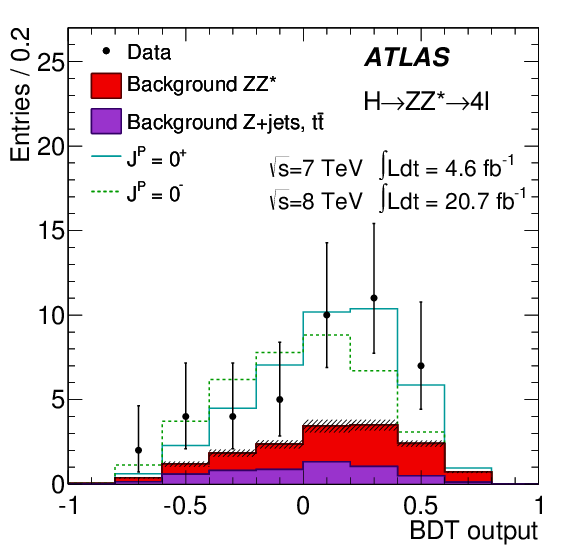
This is why, when I saw that the analysis concluded that the scalar hypothesis is supported with a probability of over 97%, I felt rather skeptical. And I thought I knew the reason: I thought that the experimental error, i.e., the error bars in the plot above, was not properly accounted for in the analysis.

Indeed, if I calculate the normalized chi-square per degree of freedom, I get \(\chi^2_{J^P=0^+} = 0.247\) and \(\chi^2_{J^P=0^-} = 0.426\), respectively, for the two hypotheses. The difference is not very big.

Alas, my skepticism was misplaced. The folks at the LHC didn’t bother with chi-squares, instead they performed a likelihood analysis. The question they were asking was this: given the set of observations available, what are the likelihoods of the scalar and the pseudoscalar scenarios?

At the LHC, they used likelihood functions and distributions derived from the actual theory. However, I can do a poor man’s version myself by simply using the Gaussian normal distribution (or a nonsymmetric version of the same). Given a data point \(D_i\), a model value \(M_I\), and a standard deviation (error) \(\sigma_i\), the probability that the data point is at least as far from \(M_i\) as \(D_i\) is given by

\begin{align}
{\cal P}_i=2\left[1-\Psi\left(\frac{|D_i-M_i|}{\sigma_i}\right)\right],
\end{align}

where \(\Psi(x)\) is the cumulative normal distribution.

Now \({\cal P}_i\) also happens to be the likelihood of the model value \(M_i\) given the data point \(D_i\) and standard distribution \(\sigma_i\). If we assume that the data points and their errors are statistically indepdendent, the likelihood that all the data points happen to fall where they fell is given by

\begin{align}
{\cal L}=\prod\limits_{i=1}^N{\cal P}_i.
\end{align}

Taking the data from the ATLAS figure above, the value \(q\) of the commonly used log-likelihood ratio is

\begin{align}
q=\ln\frac{{\cal L}(J^P=0^+)}{{\cal L}(J^P=0^-)}=2.89.
\end{align}

(The LHC folks calculated 2.2, which is “close enough” for me given that I am using a naive Gaussian distribution.)

Furthermore, if I choose to believe that the only two viable hypothesis for the spin-parity of the observed particle are the scalar and pseudoscalar scenarios (e.g., if other experiments already convinced me that alternatives, such as intepreting the result as a spin-2 particle, can be completely excluded) I can normalize these two likelihoods and interpret them as probabilities. The probability of the scalar scenario is then \(e^{2.89}\simeq 18\) times larger than the probability of the pseudoscalar scenario. So if these probabilities add up to 100%, that means that the scalar scenario is favored with a probability of nearly 95%. Not exactly “slam dunk” but pretty darn convincing.

As to the validity of the method, there is, in fact, a theorem called the Neyman-Pearson lemma that states that the likelihood-ratio test is the most powerful test for this type of comparison of hypotheses.

But what about my earlier objection that the observational error was not properly accounted for? Well… it appears that it was, after all. In my “poor man’s” version of the analysis, the observational error was used to select the appropriate form of the normal distribution, through \(\sigma_i\). In the LHC’s analysis, I believe, the observational error found its was into the Monte-Carlo simulation that was used to develop a physically more accurate probability distribution function that was used for the same purpose.

Even clever people make mistakes. Even large groups of very clever people sometimes succumb to groupthink. But when you bet against clever people, you are likely to lose. I thought I spotted an error in the analysis performed at the LHC, but all I really found were gaps in my own understanding. Oh well… live and learn.