So here I am, reading about some trivial yet not-so-trivial probability distributions.
Let’s start with the uniform distribution. Easy-peasy, isn’t it: a random number, between 0 and 1, with an equal probability assigned to any value within this range.
So… what happens if I take two such random numbers and add them? Why, I get a random number between 0 and 2 of course. But the probability distribution will no longer be uniform. There are more ways to get a value in the vicinity of 1 than near 0 or 2.
And what happens if I add three such random numbers? Or four? And so on?
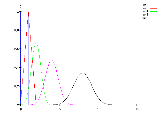
The statistics of this result are captured by the Irwin-Hall distribution, defined as
$$f_{\rm IH}(x,n)=\dfrac{1}{2(n-1)!}\sum\limits_{k=1}^n(-1)^k\begin{pmatrix}n\\k\end{pmatrix}(x-k)^{n-1}{\rm sgn}(x-k).$$
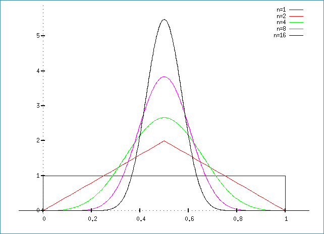
OK, so that’s what happens when we add these uniformly generated random values. What happens when we average them? This, in turn, is captured by the Bates distribution, which, unsurprisingly, is just the Irwin-Hall distribution, scaled by the factor \(n\):
$$f_{\rm B}(x,n)=\dfrac{n}{2(n-1)!}\sum\limits_{k=1}^n(-1)^k\begin{pmatrix}n\\k\end{pmatrix}(nx-k)^{n-1}{\rm sgn}(nx-k).$$
How about that.
For what it’s worth, here is the Maxima script to generate the Irwin-Hall plot:
fI(x,n):=1/2/(n-1)!*sum((-1)^k*n!/k!/(n-k)!*(x-k)^(n-1)*signum(x-k),k,0,n);
plot2d([fI(x,1),fI(x,2),fI(x,4),fI(x,8),fI(x,16)],[x,-2,18],[box,false],
       [legend,"n=1","n=2","n=4","n=8","n=16"],[y,-0.1,1.1]);
And this one for the Bates plot:
fB(x,n):=n/2/(n-1)!*sum((-1)^k*n!/k!/(n-k)!*(n*x-k)^(n-1)*signum(n*x-k),k,0,n);
plot2d([fB(x,1),fB(x,2),fB(x,4),fB(x,8),fB(x,16)],[x,-0.1,1.1],[box,false],
       [legend,"n=1","n=2","n=4","n=8","n=16"],[y,-0.1,5.9]);
Yes, I am still a little bit of a math geek at heart.