I was so busy yesterday, it was only after midnight that I realized the significance of the date.
It was exactly 40 years ago yesterday, on August 12, 1981, that IBM introduced this thing to the world:

Yes, the IBM Model 5150 personal computer, better known simply as the IBM PC.
Little did we know that this machine would change the world. In 1981, it was just one of many competing architectures, each unique, each incompatible with the rest. A program written for the Apple II could not possibly run on a Commodore VIC 20. The Sinclair ZX81 even used a different microprocessor. Between different processors, different graphics chips, different methods of sound generation, different external interfaces, each machine created its own software ecosystem. Programs that were made available for multiple architectures were essentially redeveloped from scratch, with little, if any, shared code between versions (especially since larger, more complex applications were invariably written in machine language for efficient execution).
The PC changed all that but it took a few years for that change to become evident. There were multiple factors that made this possible.
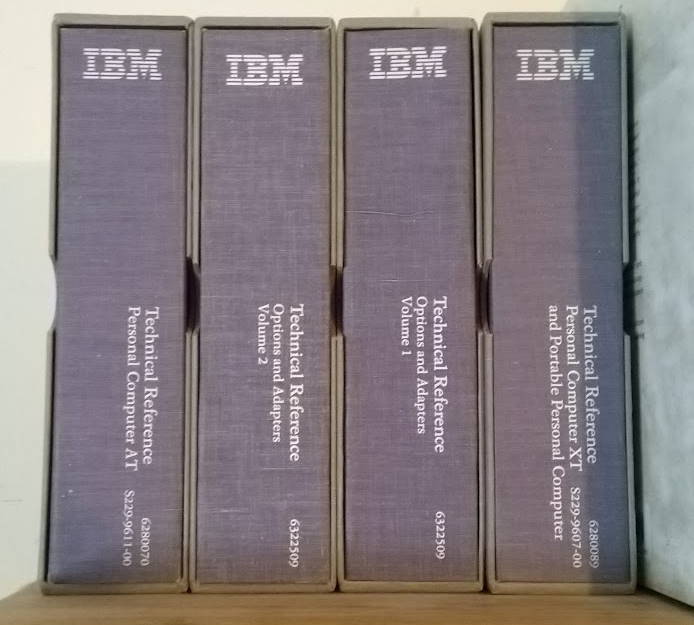
First and foremost among them, it was IBM’s decision to create a well-documented, open hardware architecture that was not protected by layers and layers of patents. The level of documentation provided by IBM was truly unprecedented in the world of personal computers. An entire series of books were offered, in traditional binders characteristic of technical documentation of the era:

As to what’s in these volumes, here’s a random page from the XT technical reference manual:

This level of detail made it possible, easy even for a hardware ecosystem to emerge: first, companies that manufactured novel extension boards for the PC and eventually, “clone” makers who built “IBM compatible” computers using “clean room” functional equivalents, developed by companies like Phoenix Technologies, of the machine’s basic software component, the BIOS (Basic Input Output System).
But the other deciding factor was the fateful decision to allow Microsoft to market their own version of the PC’s operating system, DOS. IBM’s computers came with the IBM branded version called “PC-DOS”, but Microsoft was free to sell their own, “MS-DOS”.
Thus, starting in 1984 or so, the market of IBM compatible computers was born, and it rapidly eclipsed IBM’s own market share.
And amazingly, the architecture that they created 40 years ago is still fundamentally the same architecture that we use today. OK, you may not be able to boot an MS-DOS floppy on a new machine with UEFI Secure Boot enabled, but if the BIOS permits you to turn it off, and you actually have a working floppy drive (or, more likely, a CD-ROM drive with a bootable CD image of the old operating system) you just might be in luck and boot that machine using MS-DOS 2.1, so that you can then run an early version of Lotus 1-2-3 or WordPerfect. (Of course you can run all of that in a DOSBox, but DOSBox is a software emulation of the IBM PC, so that does not really count.)
And while 64-bit versions of Windows no longer run really old 16-bit software without tools such as virtual machines or the aforementioned DOSBox, to their credit Microsoft still makes an effort to maintain robust backward compatibility: This is how I end up using a 24-year old accounting program to keep track of my personal finances, or Microsoft’s 25-year old “Bookshelf” product with an excellent, easy-to-use version of the American Heritage Dictionary. (No, I am not adverse to change or the use of newer software. But it so happens that these packages work flawlessly, do exactly what I need them to do, and so far I have not come across any replacement that delivers the functionality I need, even if I ignore all the unnecessary bloat.)
So here we are: 40 years. It’s insane. Perhaps it is worth mentioning the original, baseline specifications of the IBM 5150 Personal Computer. It has a 16-bit processor running at 0.00477 GHz. It had approximately 0.000015 gigabytes of RAM. The baseline configuration had no permanent storage, only a cassette tape interface for storing BASIC programs. The version capable of running PC-DOS had four times as much RAM, 0.000061 gigabytes, and external storage in the form of a single-sided, single-density 5.25″ floppy disk drive capable of storing 0.00034 gigabytes of data on a single disk. (Be grateful that I did not use terabytes to describe its capacity.) The computer had no real-time clock (when PC-DOS started, it asked for the time and date). Its monochrome display adapter was text only, capable of showing 25 lines by 80 characters each. Alternatively the user could opt to purchase a machine equipped with a CGA (color graphics adapter), capable of showing a whopping 16 colors at the resolution of 160 by 100 pixels, or a high resolution monochrome image at 640 by 200 pixels. Sound was provided through a simple beeper, controlled entirely by software. Optional external interfaces included RS-232 serial and IEEE 1284 parallel ports.
Compare that to the specifications of a cheap smartphone today, 40 years later.


