Physics – Page 4 – Spinor Info

Some common, naive misunderstandings in cosmology

Jan 162019

I run across this often. Well-meaning folks who read introductory-level texts or saw a few educational videos about physical cosmology, suddenly discovering something seemingly profound.

And then, instead of asking themselves why, if it is so easy to stumble upon these results, they haven’t been published already by others, they go ahead and make outlandish claims. (Claims that sometimes land in my Inbox, unsolicited.)

Let me explain what I am talking about.

As it is well known, the rate of expansion of the cosmos is governed by the famous Hubble parameter: $H\sim 70~{\rm km}/{\rm s}/{\rm Mpc}$. That is to say, two galaxies that are 1 megaparsec (Mpc, about 3 million light years) apart will be flying away from each other at a rate of 70 kilometers a second.

It is possible to convert megaparsecs (a unit of length) into kilometers (another unit of length), so that the lengths cancel out in the definition of $H$, and we are left with $H\sim 2.2\times 10^{-18}~{\rm s}^{-1}$, which is one divided by about 14 billion years. In other words, the Hubble parameter is just the inverse of the age of the universe. (It would be exactly the inverse of the age of the universe if the rate of cosmic expansion was constant. It isn’t, but the fact that the expansion was slowing down for the first 9 billion years or so and has been accelerating since kind of averages things out.)

And this, then, leads to the following naive arithmetic. First, given the age of the universe and the speed of light, we can find out the “radius” of the observable universe:

$$a=\dfrac{c}{H},$$

or about 14 billion light years. Inverting this equation, we also get $H=c/a$.

But the expansion of the cosmos is governed by another equation, the first so-called Friedmann equation, which says that

$$H^2=\dfrac{8\pi G\rho}{3}.$$

Here, \rho is the density of the universe. The mass within the visible universe, then, is calculated as usual, just using the volume of a sphere of radius $a$:

$$M=\dfrac{4\pi a^3}{3}\rho.$$

Putting this expression and the expression for $H$ back into the Friedmann equation, we get the following:

$$a=\dfrac{2GM}{c^2}.$$

But this is just the Schwarzschild radius associated with the mass of the visible universe! Surely, we just discovered something profound here! Perhaps the universe is a black hole!

Well… not exactly. The fact that we got the Schwarzschild radius is no coincidence. The Friedmann equations are, after all, just Einstein’s field equations in disguise, i.e., the exact same equations that yield the formula for the Schwarzschild radius.

Still, the two solutions are qualitatively different. The universe cannot be the interior of a black hole’s event horizon. A black hole is characterized by an unavoidable future singularity, whereas our expanding universe is characterized by a past singularity. At best, the universe may be a time-reversed black hole, i.e., a “white hole”, but even that is dubious. The Schwarzschild solution, after all, is a vacuum solution of Einstein’s field equations, wereas the Friedmann equations describe a matter-filled universe. Nor is there a physical event horizon: the “visible universe” is an observer-dependent concept, and two observers in relative motion or even two observers some distance apart, will not see the same visible universe.

Nonetheless, these ideas, memes perhaps, show up regularly, in manuscripts submitted to journals of dubious quality, appearing in self-published books, or on the alternative manuscript archive viXra. And there are further variations on the theme. For instance, the so-called Planck power, divided by the Hubble parameter, yields $2Mc^2$, i.e., twice the mass-energy in the observable universe. This coincidence is especially puzzling to those who work it out numerically, and thus remain oblivious to the fact that the Planck power is one of those Planck units that does not actually contain the Planck constant in its definition, only $c$ and $G$. People have also been fooling around with various factors of $2$, $\tfrac{1}{2}$ or $\ln 2$, often based on dodgy information content arguments, coming up with numerical ratios that supposedly replicate the matter, dark matter, and dark energy content.

Connections

Aviation, Health, History, Physics, Politics No Responses »

Jan 012019

Today, I answered a question on Quora about the nature of $c$, the speed of light, as it appears in the one equation everyone knows, $E=mc^2.$

I explained that it is best viewed as a conversion factor between our units of length and time. These units are accidents of history. There is nothing fundamental in Nature about one ten millionth the distance from the poles to the equator of the Earth (the original definition of the meter) or about one 86,400th the length of the Earth’s mean solar day. These units are what they are, in part, because we learned to measure length and time long before we learned that they are aspects of the same thing, spacetime.

And nothing stops us from using units such as light-seconds and seconds to measure space and time; in such units, the value of the speed of light would be just 1, and consequently, it could be dropped from equations altogether. This is precisely what theoretical physicists often do.

But then… I commented that something very similar takes place in aviation, where different units are used to measure horizontal distance (nautical miles, nmi) and altitude (feet, ft). So if you were to calculate the kinetic energy of an airplane (measuring its speed in nmi/s) and its potential energy (measuring the altitude, as well as the gravitational acceleration, in ft) you would need the ft/nmi conversion factor of 6076.12, squared, to convert between the two resulting units of energy.

As I was writing this answer, though, I stumbled upon a blog entry that discussed the crazy, mixed up units of measure still in use worldwide in aviation. Furlongs per fortnight may pretty much be the only unit that is not used, as just about every other unit of measure pops up, confusing poor pilots everywhere: Meters, feet, kilometers, nautical miles, statute miles, kilograms, pounds, millibars, hectopascals, inches of mercury… you name it, it’s there.

Part of the reason, of course, is the fact that America, alone among industrialized nations, managed to stick to its archaic system of measurements. Which is another historical accident, really. A lot had to do with the timing: metric transition was supposed to take place in the 1970s, governed by a presidential executive order signed by Gerald Ford. But the American economy was in a downturn, many Americans felt the nation under siege, the customary units worked well, and there was a conservative-populist pushback against the metric system… so by 1982, Ronald Reagan disbanded the Metric Board and the transition to metric was officially over. (Or not. The metric system continues to gain ground, whether it is used to measure bullets or Aspirin, soft drinks or street drugs.)

Yet another example similar to the metric system is the historical accident that created the employer-funded healthcare system in the United States that American continue to cling to, even as most (all?) other advanced industrial nations transitioned to something more modern, some variant of a single-payer universal healthcare system. It happened in the 1920s, when a Texas hospital managed to strike a deal with public school teachers in Dallas: For 50 cents a month, the hospital picked up the tab of their hospital visits. This arrangement became very popular during the Great Depression when hospitals lost patients who could not afford their hospital care anymore. The idea came to be known as Blue Cross. And that’s how the modern American healthcare system was born.

As I was reading this chain of Web articles, taking me on a tour from Einstein’s $E=mc^2$ to employer-funded healthcare in America, I was reminded of a 40-year old British TV series, Connections, created by science historian James Burke. Burke found similar, often uncanny connections between seemingly unrelated topics in history, particularly the history of science and technology.

Another Perimeter visit

Personal, Physics No Responses »

Oct 182018

Just got back from The Perimeter Institute, where I spent three very short days.

I had good discussions with John Moffat. I again met Barak Shoshany, whom I first encountered on Quora. I attended two very interesting and informative seminar lectures by Emil Mottola on quantum anomalies and the conformal anomaly.

I also gave a brief talk about our research with Slava Turyshev on the Solar Gravitational Lens. I was asked to give an informal talk with no slides. It was a good challenge. I believe I was successful. My talk seemed well received. I was honored to have Neil Turok in the audience, who showed keen interest and asked several insightful questions.

Congratulations, Donna Strickland

Canada, Physics No Responses »

Oct 022018

I just watched a news conference held by the University of Waterloo, on account of Donna Strickland being awarded the Nobel prize in physics.

This is terrific news for Canada, for the U. of Waterloo, and last but most certainly not least, for women in physics.

Heartfelt congratulations!

Atiyah, Riemann and the fine structure constant

Mathematics, Physics No Responses »

Sep 252018

Michael Atiyah, 89, is one of the greatest living mathematicians. Which is why the world pays attention when he claims to have solved what is perhaps the greatest outstanding problem in mathematics, the Riemann hypothesis.

Here is a simple sum: $1+\frac{1}{2^2}+\frac{1}{3^2}+…$. It is actually convergent: The result is $\pi^2/6$.

Other, similar sums also converge, so long as the exponent is greater than 1. In fact, we can define a function:

$$\begin{align*}\zeta(x)=\sum\limits_{i=1}^\infty\frac{1}{i^x}.\end{align*}$$

Where things get really interesting is when we extend the definition of this $\zeta(x)$ to the entire complex plane. As it turns out, its analytic continuation is defined almost everywhere. And, it has a few zeros, i.e., values of $x$ for which $\zeta(x)=0$.

The so-called trivial zeros of $\zeta(x)$ are the negative even integers: $x=-2,-4,-6,…$. But the function also has infinitely many nontrivial zeros, where $x$ is complex. And here is the thing: The real part of all known nontrivial zeros happens to be $\frac{1}{2}$, the first one being at $x=\frac{1}{2}+14.1347251417347i$. This, then, is the Riemann hypothesis: Namely that if $x$ is a non-trivial zero of $\zeta(x)$, then $\Re(x)=\frac{1}{2}$. This hypothesis baffled mathematicians for the past 130 years, and now Atiyah claims to have solved it, accidentally (!), in a mere five pages. Unfortunately, verifying his proof is above my pay grade, as it references other concepts that I would have to learn first. But it is understandable why the mathematical community is skeptical (to say the least).

A slide from Atiyah’s talk on September 24, 2018.

What is not above my pay grade is analyzing Atiyah’s other claim: a purported mathematical definition of the fine structure constant $\alpha$. The modern definition of $\alpha$ relates this number to the electron charge $e$: $\alpha=e^2/4\pi\epsilon_0\hbar c$, where $\epsilon_0$ is the electric permeability of the vacuum, $\hbar$ is the reduced Planck constant and $c$ is the speed of light. Back in the days of Arthur Eddington, it seemed that $\alpha\sim 1/136$, which led Eddington himself onto a futile quest of numerology, trying to concoct a reason why $136$ is a special number. Today, we know the value of $\alpha$ a little better: $\alpha^{-1}\simeq 137.0359992$.

Atiyah produced a long and somewhat rambling paper that fundamentally boils down to two equations. First, he defines a new mathematical constant, denoted by the Cyrillic letter $\unicode{x427}$ (Che), which is related to the fine structure constant by the equation

$$\begin{align*}\alpha^{-1}=\frac{\pi\unicode{x427}}{\gamma},\tag{1.1*}\end{align*}$$

where $\gamma=0.577…$ is the Euler–Mascheroni constant. Second, he offers a definition for $\unicode{x427}$:

$$\begin{align*}\unicode{x427}=\frac{1}{2}\sum\limits_{j=1}^\infty 2^{-j}\left(1-\int_{1/j}^j\log_2 x~dx\right).\tag{7.1*}\end{align*}$$

(The equation numbers are Atiyah’s; I used a star to signify that I slightly simplified them.)

Atiyah claims that this sum is difficult to calculate and then goes into a long-winded and not very well explained derivation. But the sum is not difficult to calculate. In fact, I can calculate it with ease as the definite integral under the summation sign is trivial:

$$\begin{align*}\int_{1/j}^j\log_2 x~dx=\frac{(j^2+1)\log j-j^2+1}{j\log 2}.\end{align*}$$

After this, the sum rapidly converges, as this little bit of Maxima code demonstrates (NB: for $j=1$ the integral is trivial as the integration limits collapse):

(%i1) assume(j>1);
(%o1)                               [j > 1]
(%i2) S:1/2*2^(-j)*(1-integrate(log(x)/log(2),x,1/j,j));
                                  log(j) + 1
                                  ---------- + j log(j) - j
                   (- j) - 1          j
(%o2)             2          (1 - -------------------------)
                                           log(2)
(%i3) float(sum(S,j,1,50));
(%o3)                         0.02944508691740671
(%i4) float(sum(S,j,1,100));
(%o4)                         0.02944508691730876
(%i5) float(sum(S,j,1,150));
(%o5)                         0.02944508691730876
(%i6) float(sum(S,j,1,100)*%pi/%gamma);
(%o6)                         0.1602598029967022

Unfortunately, this does not look like $\alpha^{-1}=137.0359992$ at all. Not even remotely.

So we are all left to guess, sadly, what Atiyah was thinking when he offered this proposal.

We must also remember that $\alpha$ is a so-called “running” constant, as its value depends on the energy of the interaction, though presumably, the constant in question here is $\alpha$ in the infrared limit, i.e., at zero energy.

Sterile neutrinos? Not so fast…

Physics No Responses »

Jun 032018

I am reading some breathless reactions to a preprint posted a few days ago by the MiniBooNE experiment. The experiment is designed to detect neutrinos, in particular neutrino oscillations (the change of one neutrino flavor into another.)

The headlines are screaming. Evidence found of a New Fundamental Particle, says one. Strange New Particle Could Prove Existence of Dark Matter, says another. Or how about, A Major Physics Experiment Just Detected A Particle That Shouldn’t Exist?

The particle in question is the so-called sterile neutrino. It is a neat concept, one I happen to quite like. It represents an elegant resolution to the puzzle of neutrino handedness. This refers to the chirality of neutrinos, essentially the direction in which they spin compared to their direction of motion. We only ever see “left handed” neutrinos. But neutrinos have rest mass. So they move slower than light. That means that if you run fast enough and outrun a left-handed neutrino, so that relative to you it is moving backwards (but still spins in the same direction as before), when you look back, you’ll see a right-handed neutrino. This implies that right-handed neutrinos should be seen just as often as left-handed neutrinos. But they aren’t. How come?

Sterile neutrinos offer a simple answer: We don’t see right-handed neutrinos because they don’t interact (they are sterile). That is to say, when a neutrino interacts (emits or absorbs a Z-boson, or emits or absorbs a W-boson while changing into a charged lepton), it has to be a left-handed neutrino in the interaction’s center-of-mass frame.

If this view is true and such sterile neutrinos exist, even though they cannot be detected directly, their existence would skew the number of neutrino oscillation events. As to what neutrino oscillations are: neutrinos are massive. But unlike other elementary particles, neutrinos do not have a well-defined mass associated with their flavor (electron, muon, or tau neutrino). When a neutrino has a well-defined flavor (is in a flavor eigenstate) it has no well-defined mass and vice versa. This means that if we detect neutrinos in a mass eigenstate, their flavor can appear to change (oscillate) between one state or another; e.g., a muon neutrino may appear at the detector as an electron neutrino. These flavor oscillations are rare, but they can be detected, and that’s what the MiniBooNE experiment is looking for.

And that is indeed what MiniBooNE found: an excess of events that is consistent with neutrino oscillations.

MiniBooNE detects electron neutrinos. These can come from all kinds of (background) sources. But one particular source is an intense beam of muon neutrinos produced at Fermilab. Because of neutrino oscillations, some of the neutrinos in this beam will be detected as electron neutrinos, yielding an excess of electron neutrino events above background.

And that’s exactly what MiniBooNE sees, with very high confidence: 4.8σ. That’s almost the generally accepted detection threshold for a new particle. But this value of 4.8σ is not about a new particle. It is the significance associated with excess electron neutrino detection events overall: an excess that is expected from neutrino oscillations.

So what’s the big deal, then? Why the screaming headlines? As far as I can tell, it all boils down to this sentence in the paper: “Although the data are fit with a standard oscillation model, other models may provide better fits to the data.”

What this somewhat cryptic sentence means is best illustrated by a figure from the paper:

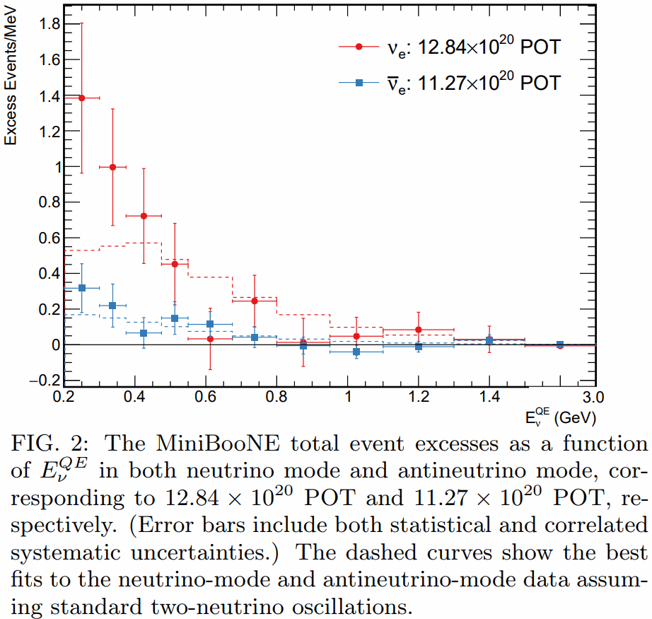
This figure shows the excess events (above background) detected by MiniBooNE, but also the expected number of excess events from neutrino oscillations. Notice how only the first two red data points fall significantly above the expected number. (In case you are wondering, POT means Protons On Target, that is to say, the number of protons hitting a beryllium target at Fermilab, producing the desired beam of muon neutrinos.)

Yes, these two data points are intriguing. Yes, they may indicate the existence of new physics beyond two-neutrino oscillations. In particular, they may indicate the existence of another oscillation mode, muon neutrinos oscillating into sterile neutrinos that, in turn, oscillate into electron neutrinos, yielding this excess.

Mind you, if this is a sign of sterile neutrinos, these sterile neutrinos are unlikely dark matter candidates; their mass would be too low.

Or these two data points are mere statistical flukes. After all, as the paper says, “the best oscillation fit to the excess has a probability of 20.1%”. That is far from improbable. Sure, the fact that it is only 20.1% can be interpreted as a sign of some tension between the Standard Model and this experiment. But it is certainly not a discovery of new physics, and absolutely not a confirmation of a specific model of new physics, such as sterile neutrinos.

And indeed, the paper makes no such claim. The word “sterile” appears only four times in the paper, in a single sentence in the introduction: “[…] more exotic models are typically used to explain these anomalies, including, for example, 3+N neutrino oscillation models involving three active neutrinos and N additional sterile neutrinos [6-14], resonant neutrino oscillations [15], Lorentz violation [16], sterile neutrino decay [17], sterile neutrino non-standard interactions [18], and sterile neutrino extra dimensions [19].”

So yes, there is an intriguing sign of an anomaly. Yes, it may point the way towards new physics. It might even be new physics involving sterile neutrinos.

But no, this is not a discovery. At best, it’s an intriguing hint; quite possibly, just a statistical fluke.

So why the screaming headlines, then? I wish I knew.

Comoving distance

Astronomy, Physics 10 Responses »

May 292018

There is an excellent diagram accompanying an answer on StackExchange, and I’ve been meaning to copy it here, because I keep losing the address.

The diagram summarizes many measures of cosmic expansion in a nice, compact, but not necessarily easy-to-understand form:

So let me explain how to read this diagram. First of all, time is going from bottom to top. The thick horizontal black line represents the moment of now. Imagine this line moving upwards as time progresses.

The thick vertical black line is here. So the intersection of the two thick black lines in the middle is the here-and-now.

Distances are measured in terms of the comoving distance, which is basically telling you how far a distant object would be now, if you had a long measuring tape to measure its present-day location.

The area shaded red (marked “past light cone”) is all the events that happened in the universe that we could see, up to the moment of now. The boundary of this area is everything in this universe from which light is reaching us right now.

So just for fun, let us pick an object at a comoving distance of 30 gigalightyears (Gly). Look at the dotted vertical line corresponding to 30 Gly, halfway between the 20 and 40 marks (either side, doesn’t matter.) It intersects the boundary of the past light cone when the universe was roughly 700 million years old. Good, there were already young galaxies back then. If we were observing such a galaxy today, we’d be seeing it as it appeared when the universe was 700 million years old. Its light would have spent 13.1 billion years traveling before reaching our instruments.

Again look at the dotted vertical line at 30 Gly and extend it all the way to the “now” line. What does this tell you about this object? You can read the object’s redshift (z) off the diagram: its light is shifted down in frequency by a factor of about 9.

You can also read the object’s recession velocity, which is just a little over two times the vacuum speed of light. Yes… faster than light. This recession velocity is based on the rate of change of the scale factor, essentially the Hubble parameter times the comoving distance. The Doppler velocity that one would deduce from the object’s redshift yields a value less than the vacuum speed of light. (Curved spacetime is tricky; distances and speeds can be defined in various ways.)

Another thing about this diagram is that in addition to the past, it also sketches the future, taking into account the apparent accelerating expansion of the universe. Notice the light red shaded area marked “event horizon”. This area contains everything that we will be able to see at our present location, throughout the entire history of the universe, all the way to the infinite future. Things (events) outside this area will never be seen by us, will never influence us.

Note how the dotted line at 30 Gly intersects this boundary when the universe is about 5 billion years old. Yes, this means that we will only ever see the first less than 5 billion years of existence of a galaxy at a comoving distance of 30 Gly. Over time, light from this galaxy will be redshifted ever more, until it eventually appears to “freeze” and disappears from sight, never appearing to become older than 5 billion years.

Notice also how the dashed curves marking constant values of redshift bend inward, closer and closer to the “here” location as we approach the infinite future. This is a direct result of accelerating expansion: Things nearer and nearer to us will be caught up in the expansion, accelerating away from our location. Eventually this will stop, of course; cosmic acceleration will not rip apart structures that are gravitationally bound. But we will end up living in a true “island universe” in which nothing is seen at all beyond the largest gravitationally bound structure, the local group of galaxies. Fortunately that won’t happen anytime soon; we have many tens of billions of years until then.

Lastly, the particle horizon (blue lines) essentially marks the size of the visible part of the universe at any given time. Notice how the width of the interval marked by the intersection of the now line and the blue lines is identical to the width of the past light cone at the bottom of this diagram. Notice also how the blue lines correspond to infinite redshift.

As I said, this diagram is not an easy read but it is well worth studying.

Hawking again

Physics No Responses »

Apr 232018

Stephen Hawking passed away over a month ago, but I just came across this beautiful tribute from cartoonist Sean Delonas. It was completely unexpected (I was flipping through the pages of a magazine) and, I admit, it had quite an impact on me. Not the words, inspirational though they may be… the image. The empty wheelchair, the frail human silhouette walking away in the distance.

Modified gravity and NGC1052-DF2

Physics No Responses »

Apr 022018

The recent discovery of a galaxy, NGC1052-DF2, with no or almost no dark matter made headlines worldwide.

Nature 555, 629–632 (29 March 2018)

Somewhat paradoxically, it has been proclaimed by some as evidence that the dark matter paradigm prevails over theories of modified gravity. And, as usual, many of the arguments were framed in the context of dark matter vs. MOND, as if MOND was a suitable representative of all modified gravity theories. One example is a recent Quora question, Can we say now that all MOND theories is proven false, and there is really dark matter after all? I offered the following in response:

First of all, allow me to challenge the way the question is phrased: “all MOND theories”… Please don’t.

MOND (MOdified Newtonian Dynamics) is not a theory. It is an ad hoc, phenomenological replacement of the Newtonian acceleration law with a simplistic formula that violates even basic conservation laws. The formula fits spiral galaxy rotation curves reasonably well, consistent with the empirical Tully—Fisher law that relates galaxy masses and rotational velocities, but it fails for just about everything else, including low density globular clusters, dwarf galaxies, clusters of galaxies, not to mention cosmological observations.

MOND was given a reprieve in the form of Jacob Beckenstein’s TeVeS (Tensor—Vector—Scalar gravity), which is an impressive theoretical exercise to create a proper classical field theory that reproduces the MOND acceleration law in the weak field, low velocity limit. However, TeVeS suffers from the same issues MOND does when confronted with data beyond galaxy rotation curves. Moreover, the recent gravitational wave event, GW170817, accompanied by the gamma ray burst GRB170817 from the same astrophysical event, thus demonstrating that the propagation speed of gravitational and electromagnetic waves is essentially identical, puts all bimetric theories (of which TeVeS is an example) in jeopardy.

But that’s okay. News reports suggesting the death of modified gravity are somewhat premature. While MOND has often been used as a straw man by opponents of modified gravity, there are plenty of alternatives, many of them much better equipped than MOND to deal with diverse astrophysical phenomena. For instance, f(R) gravity, entropic gravity, Horava—Lifshitz gravity, galileon theory, DGP (Dvali—Gabadadze—Porrati) gravity… The list goes on and on. And yes, it also includes John Moffat’s STVG (Scalar—Tensor—Vector Gravity — not to be confused with TeVeS, the two are very different animals) theory, better known as MOG, a theory to which I also contributed.

As to NGC1052-DF2, for MOG that’s actually an easy one. When you plug in the values for the MOG approximate solution that we first published about a decade ago, you get an effective dynamical mass that is less than twice the visible (baryonic) mass of this galaxy, which is entirely consistent with its observed velocity dispersion.

In fact, I’d go so far as to boldly suggest that NGC1052-DF2 is a bigger challenge for the dark matter paradigm than it is for some theories of modified gravity (MOG included). Why? Because there is no known mechanism that would separate dark matter from stellar mass.

Compare this to the infamous Bullet Cluster: a pair of galaxy clusters that have undergone a collision. According to the explanation offered within the context of the dark matter paradigm (NB: Moffat and Brownstein showed, over a decade ago, that the Bullet Cluster can also be explained without dark matter, using MOG), their dark matter halos just flew through each other without interaction (other than gravity), as did the stars (stars are so tiny compared to the distance between them, the likelihood of stellar collisions is extremely remote, so stars also behave like a pressureless medium, like dark matter.) Interstellar/intergalactic clouds of gas, however, did collide, heating up to millions of degrees (producing bright X-rays) and losing much of their momentum. So you end up with a cloud of gas (but few stars and little dark matter) in the middle, and dark matter plus stars (but little gas) on the sides. This separation process works because stars and dark matter behave like a pressureless medium, whereas gas does not.

But in the case of NGC1052-DF2, some mechanism must have separated stars from dark matter, so we end up with a galaxy (one that actually looks nice, with no signs of recent disruption). I do not believe that there is currently a generally accepted, viable candidate mechanism that could accomplish this.

RIP Stephen Hawking

Physics No Responses »

Mar 142018

Stephen Hawking died earlier today.

Hawking was diagnosed with ALS in the year I was born, in 1963.

Defying his doctor’s predictions, he refused to die after a few years. Instead, he carried on for another astonishing 55 years, living a full life.

Public perception notwithstanding, he might not have been the greatest living physicist, but he was certainly a great physicist. The fact that he was able to accomplish so much despite his debilitating illness made him an extraordinary human being, a true inspiration.

Here is a short segment, courtesy of CTV Kitchener, filmed earlier today at the Perimeter Institute. My friend and colleague John Moffat, who met Hawking many times, is among those being interviewed:

The Solar Gravitational Telescope

Astronomy, Personal, Physics, Space No Responses »

Mar 102018

There is a very interesting concept in the works at NASA, to which I had a chance to contribute a bit: the Solar Gravitational Telescope.

The idea, explained in this brand new NASA video, is to use the bending of light by the Sun to form an image of distant objects.

The resolving power of such a telescope would be phenomenal. In principle, it is possible to use it to form a megapixel-resolution image of an exoplanet as far as 100 light years from the Earth.

The technical difficulties are, however, challenging. For starters, a probe would need to be placed at least 550 astronomical units (about four times the distance to Voyager 1) from the Sun, precisely located to be on the opposite side of the Sun relative to the exoplanet. The probe would then have to mimic the combined motion of our Sun (dragged about by the gravitational pull of planets in the solar system) and the exoplanet (orbiting its own sun). Light from the Sun will need to be carefully blocked to ensure that we capture light from the exoplanet with as little noise as possible. And each time the probe takes a picture of the ring of light (the Einstein ring) around the Sun, it will be the combined light of many adjacent pixels on the exoplanet. The probe will have traverse a region that is roughly a kilometer across, taking pictures one pixel at a time, which will need to be deconvoluted. The fact that the exoplanet itself is not constant in appearance (it will go through phases of illumination, it may have changing cloud cover, perhaps even changes in vegetation) further complicates matters. Still… it can be done, and it can be accomplished using technology we already have.

By its very nature, it would be a very long duration mission. If such a probe was launched today, it would take 25-30 years for it to reach the place where light rays passing on both sides of the Sun first meet and thus the focal line begins. It will probably take another few years to collect enough data for successful deconvolution and image reconstruction. Where will I be 30-35 years from now? An old man (or a dead man). And of course no probe will be launched today; even under optimal circumstances, I’d say we’re at least a decade away from launch. In other words, I have no chance of seeing that high-resolution exoplanet image unless I live to see (at least) my 100th birthday.

Still, it is fun to dream, and fun to participate in such things. Though now I better pay attention to other things as well, including things that, well, help my bank account, because this sure as heck doesn’t.

And the answer is: Momentum conservation

Physics No Responses »

Jan 302018

I was surprised by the number of people who found my little exercise about kinetic energy interesting.

However, I was disappointed by the fact that only one person (an astrophysicist by trade) got it right.

It really isn’t a very difficult problem! You just have to remember that in addition to energy, momentum is also conserved.

In other words, when a train accelerates, it is pushing against something… the Earth, that is. So ever so slightly, the Earth accelerates backwards. The change in velocity may be tiny, but the change in energy is not necessarily so. It all depends on your reference frame.

So let’s do the math, starting with a train of mass $m$ that accelerates from $v_1$ to $v_2$. (Yes, I am doing the math formally; we can plug in the actual numbers in the end.)

Momentum is of course velocity times mass. Momentum conversation means that the Earth’s speed will change as

\[\Delta v = -\frac{m}{M}(v_2-v_1),\]

where $M$ is the Earth’s mass. If the initial speed of the earth is $v_0$, the change in its kinetic energy will be given by

\[\frac{1}{2}M\left[(v_0+\Delta v)^2-v_0^2\right]=\frac{1}{2}M(2v_0\Delta v+\Delta v^2).\]

If $v_0=0$, this becomes

\[\frac{1}{2}M\Delta v^2=\frac{m^2}{M}(v_2-v_1)^2,\]

which is very tiny if $m\ll M$. However, if $|v_0|>0$ and comparable in magnitude to $v_2-v_1$ (or at least, $|v_0|\gg|\Delta v|$), we get

\[\frac{1}{2}M(2v_0\Delta v+\Delta v^2)=-mv_0(v_2-v_1)+\frac{m^2}{2M}(v_2-v_1)^2\simeq -mv_0(v_2-v_1).\]

Note that the actual mass of the Earth doesn’t even matter; we just used the fact that it’s much larger than the mass of the train.

So let’s plug in the numbers from the exercise: $m=10000~{\rm kg}$, $v_0=-10~{\rm m}/{\rm s}$ (negative, because relative to the moving train, the Earth is moving backwards), $v_2-v_1=10~{\rm m}/{\rm s}$, thus $-mv_0(v_2-v_1)=1000~{\rm kJ}$.

So the missing energy is found as the change in the Earth’s kinetic energy in the reference frame of the second moving train.

Note that in the reference frame of someone standing on the Earth, the change in the Earth’s kinetic energy is imperceptibly tiny; all the $1500~{\rm kJ}$ go into accelerating the train. But in the reference frame of the observer moving on the second train on the parallel tracks, only $500~{\rm kJ}$ goes into the kinetic energy of the first train, whereas $1000~{\rm kJ}$ is added to the Earth’s kinetic energy. But in both cases, the total change in kinetic energy, $1500~{\rm kJ}$, is the same and consistent with the readings of the electricity power meter.

Then again… maybe the symbolic calculation is too abstract. We could have done it with numbers all along. When a $10000~{\rm kg}$ train’s speed goes from $10~{\rm m}/{\rm s}$ to $20~{\rm m}/{\rm s}$, it means that the $6\times 10^{24}~{\rm kg}$ Earth’s speed (in the opposite direction) will change by $10000\times 10/(6\times 10^{24})=1.67\times 10^{-20}~{\rm m}/{\rm s}$.

In the reference frame in which the Earth is at rest, the change in kinetic energy is $\tfrac{1}{2}\times (6\times 10^{24})\times (1.67\times 10^{-20})^2=8.33\times 10^{-16}~{\rm J}$.

However, in the reference frame in which the Earth is already moving at $10~{\rm m}/{\rm s}$, the change in kinetic energy is $\tfrac{1}{2}\times (6\times 10^{24})\times (10+1.67\times 10^{-20})^2-\tfrac{1}{2}\times (6\times 10^{24})\times 10^2$${}=\tfrac{1}{2}\times (6\times 10^{24})\times[2\times 10\times 1.67\times 10^{-20}+(1.67\times 10^{-20})^2] $${}\simeq 1000~{\rm kJ}$.

Kinetic energy

Physics No Responses »

Jan 272018

Enough blogging about personal stuff like our cats. Here is a neat little physics puzzle instead.

Solving this question requires nothing more than elementary high school physics (assuming you were taught physics in high school; if not, shame on the educational system where you grew up). No tricks, no gimmicks, no relativity theory, no quantum mechanics, just a straightforward application of what you were taught about Newtonian physics.

We have two parallel rail tracks. There is no friction, no air resistance, no dissipative forces.

On the first track, let’s call it A, there is a train. It weighs 10,000 kilograms. It is accelerated by an electric motor from 0 to 10 meters per second. Its kinetic energy, when it is moving at $v=10~{\rm m/s}$, is of course $K=\tfrac{1}{2}mv^2=500~{\rm kJ}$.

Next, we accelerate it from 10 to 20 meters per second. At $v=20~{\rm m/s}$, its kinetic energy is $K=2000~{\rm kJ}$, so an additional $1500~{\rm kJ}$ was required to achieve this change in speed.

All this is dutifully recorded by a power meter that measures the train’s electricity consumption. So far, so good.

But now let’s look at the B track, where there is a train moving at the constant speed of $10~{\rm m/s}$. When the A train is moving at the same speed, the two trains are motionless relative to each other; from B‘s perspective, the kinetic energy of A is zero. And when A accelerates to $20~{\rm m/s}$ relative to the ground, its speed relative to B will be $10~{\rm m/s}$; so from B‘s perspective, the change in kinetic energy is $500~{\rm kJ}$.

But the power meter is not lying. It shows that the A train used $1500~{\rm kJ}$ of electrical energy.

Question: Where did the missing $1000~{\rm kJ}$ go?

First one with the correct answer gets a virtual cookie.

GW170817 is a big freaking deal

Astronomy, Physics No Responses »

Oct 162017

Today, a “multi-messenger” observation of a gravitational wave event was announced.

This is a big freaking deal. This is a Really Big Freaking Deal. For the very first time, ever, we observed an event, the merger of two neutron stars, simultaneously using both gravitational waves and electromagnetic waves, the latter including light, radio waves, UV, X-rays, gamma rays.

From http://iopscience.iop.org/article/10.3847/2041-8213/aa91c9

The significance of this observation must not be underestimated. For the first time, we have direct validation of a LIGO gravitational wave observation. It demonstrates that our interpretation of LIGO data is actually correct, as is our understanding of neutron star mergers; one of the most important astrophysical processes, as it is one of the sources of isotopes heavier than iron in the universe.

Think about it… every time you hold, say, a piece of gold in your hands, you are holding something that was forged in an astrophysical event like this one billions of years ago.

Gravitational wave astronomy has arrived

Astronomy, Physics No Responses »

Sep 272017

So here it is: another gravitational wave event detection by the LIGO observatories. But this time, there is a twist: a third detector, the less sensitive European VIRGO observatory, also saw this event.

This is amazing. Among other things, having three observatories see the same event is sufficient to triangulate the sky position of the event with much greater precision than before. With additional detectors coming online in the future, the era of gravitational wave astronomy has truly arrived.

Video about the Solar Gravitational Telescope

Astronomy, Personal, Physics, Space 1 Response »

Jul 272017

There is a brand new video on YouTube today, explaining the concept of the Solar Gravitational Telescope concept:

It really is very well done. Based in part on our paper with Slava Turyshev, it coherently explains how this concept would work and what the challenges are. Thank you, Jimiticus.

But the biggest challenge… this would be truly a generational effort. I am 54 this year. Assuming the project is greenlighted today and the spacecraft is ready for launch in ten years’ time… the earliest for useful data to be collected would be more than 40 years from now, when, unless I am exceptionally lucky with my health, I am either long dead already, or senile in my mid-90s.

The Solar Gravitational Telescope

Personal, Physics No Responses »

Jul 132017

Slava Turyshev and I just published a paper in Physical Review. It is a lengthy, quite technical paper about the wave-theoretical treatment of the solar gravitational telescope.

What, you say?

Well, simple: using the Sun as a gravitational telescope to image distant objects. Like other stars, the Sun bends light, too. Measuring this bending of light was, in fact, the crucial test carried out by Eddington during the 1919 solar eclipse, validating the predictions of general relativity and elevating Albert Einstein to the status of international science superstar.

The gravitational bending of light is very weak. Two rays, passing on opposite sides of the Sun, are bent very little. So little in fact, it takes some 550 astronomical units (AU; the distance between the Earth and the Sun) for the two rays to meet. But where they do, interesting things happen.

If you were floating in space at that distance, and there was a distant planet on the exact opposite side of the Sun, light from a relatively small section of that planet would form a so-called Einstein ring around the Sun. The light amplification would be tremendous; a factor of tens of billions, if not more.

But you have to be located very precisely at the right spot to image a particular spot on the exoplanet. How precisely? Well, that’s what we set out to figure out, based in part on the existing literature on the subject. (Short answer: it’s measured in tens of centimeters or less.)

In principle, a spacecraft at this distance, moving slowly in lateral directions to scan the image plane (which is several kilometers across), can obtain a detailed map of a distant planet. It is possible, in principle, to obtain a megapixel resolution image of a planet dozens of light years from here, though image reconstruction would be a task of considerable complexity, due in part to the fact that an exoplanet is a moving, changing target with variable illumination and possibly cloud cover.

Mind you, getting to 550 AU is costly. Our most distant spacecraft to date, Voyager 1, is just under 140 AU from the Sun, and it took that spacecraft 40 years to get there. That said, it is a feasible mission concept, but we must be very certain that we understand the physics thoroughly.

This is where our paper comes in: an attempt to derive detailed results about how light waves pass on both sides of the Sun and recombine along the focal line.

The bulk of the work in this paper is Slava’s, but I was proud to help. Part of my contribution was to provide a visualization of the qualitative behavior of the wavefront (described by a hypergeometric function):

In this image, a light wave, initially a plane wave, travels from left to right and it is deflected by a gravitational source at the center. If you squint just a little, you can actually see a concentric circular pattern overlaid on top of the distorted wavefront. The deflection of the wavefront and this spherical wave perturbation are both well described by an approximation. However, that approximation breaks down specifically in the region of interest, namely the focal line:

The top left of these plots show the approximation of the deflected wavefront; the top right, the (near) circular perturbation. Notice how both appear to diverge along the focal line: the half line between the center of the image and the right-hand side. The bottom right plot shows the combination of the two approximations; it is similar to the full solution, but not identical. The difference between the full solution and this approximation is shown in the bottom left plot.

I also helped with working out evil-looking things like a series approximation of the confluent hypergeometric function using so-called Pochhammer symbols and Stirling numbers. It was fun!

To make a long story short, although it involved some frustratingly long hours at a time when I was already incredibly busy, it was fun, educational, and rewarding, as we gave birth to a 39-page monster (43 pages on the arXiv) with over 300 equations. Hopefully just one of many contributions that, eventually (dare I hope that it will happen within my lifetime?) may result in a mission that will provide us with a detailed image of a distant, life-bearing cousin of the Earth.

Deja vu

Cybernetics, Physics 4 Responses »

Mar 172017

Recently, I answered a question on Quora on the possibility that we live in a computer simulation.

Apparently, this is a hot topic. The other day, there was an essay on it by Sabine Hossenfelder.

I agree with Sabine’s main conclusion, as well as her point that “the programmer did it” is no explanation at all: it is just a modern version of mythology.

I also share her frustration, for instance, when she reacts to the nonsense from Stephen Wolfram about a “whole civilization” “down at the Planck scale”.

Sabine makes a point that discretization of spacetime might conflict with special relativity. I wonder if the folks behind doubly special relativity might be inclined to offer a thought or two on this topic.

In any case, I have another reason why I believe we cannot possibly live in a computer simulation.

My argument hinges on an unproven conjecture: My assumption that scalable quantum computing is really not possible because of the threshold theorem. Most supporters of quantum computing believe, of course, that the threshold theorem is precisely what makes quantum computing possible: if an error-correcting quantum computer reaches a certain threshold, it can emulate an arbitrary precision quantum computer accurately.

But I think this is precisely why the threshold will never be reached. One of these days, someone will prove a beautiful theorem that no large-scale quantum computer will ever be able to operate above the threshold, hence scalable quantum computing is just not possible.

Now what does this have to do with us living in a simulation? Countless experiments show that we live in a fundamentally quantum world. Contrary to popular belief (and many misguided popularizations) it does not mean a discretization at the quantum level. What it does mean is that even otherwise discrete quantities (e.g., the two spin states of an electron) turn into continuum variables (the phase of the wavefunction).

This is precisely what makes a quantum computer powerful: like an analog computer, it can perform certain algorithms more effectively than a digital computer, because whereas a digital computer operates on the countable set of discrete digits, a quantum or analog computer operates with the uncountable infinite of states offered by continuum variables.

Of course a conventional analog computer is very inaccurate, so nobody seriously proposed that one could ever be used to factor 1000-digit numbers.

This quantum world in which we live, with its richer structure, can be simulated only inefficiently using a digital computer. If that weren’t the case, we could use a digital computer to simulate a quantum computer and get on with it. But this means that if the world is a simulation, it cannot be a simulation running on a digital computer. The computer that runs the world has to be a quantum computer.

But if quantum computers do not exist… well, then they cannot simulate the world, can they?

Two further points about this argument. First, it is purely mathematical: I am offering a mathematical line of reasoning that no quantum universe can be a simulated universe. It is not a limitation of technology, but a (presumed) mathematical truth.

Second, the counterargument has often been proposed that perhaps the simulation is set up so that we do not get to see the discrepancies caused by inefficient simulation. I.e., the programmer cheats and erases the glitches from our simulated minds. But I don’t see how that could work either. For this to work, the algorithms employed by the simulation must anticipate not only all the possible ways in which we could ascertain the true nature of the world, but also assess all consequences of altering our state of mind. I think it quickly becomes evident that this really cannot be done without, well, simulating the world correctly, which is what we were trying to avoid… so no, I do not think it is possible.

Of course if tomorrow, someone announces that they cracked the threshold theorem and full-scale, scalable quantum computing is now reality, my argument goes down the drain. But frankly, I do not expect that to happen.

Trace-free gravity

Physics No Responses »

Jan 202017

Enough blogging about politics. It’s time to think about physics. Been a while since I last did that.

A Facebook post by Sabine Hossenfelder made me look at this recent paper by Josset et al. Indeed, the post inspired me to create a meme:

The paper in question contemplates the possibility that “dark energy”, i.e., the mysterious factor that leads to the observed accelerating expansion of the cosmos, is in fact due to a violation of energy conservation.

Sounds kooky, right? Except that the violation that the authors consider is a very specific one.

Take Einstein’s field equation,

$$R_{\mu\nu}-\tfrac{1}{2}Rg_{\mu\nu}+\Lambda g_{\mu\nu}=8\pi GT_{\mu\nu},$$

and subtract from it a quarter of its trace times the metric. The trace of the left-hand side is $-R+4\Lambda$, the right-hand side is $8\pi GT$, so we get

$$R_{\mu\nu}-\tfrac{1}{4}Rg_{\mu\nu}=8\pi G(T_{\mu\nu}-\tfrac{1}{4}Tg_{\mu\nu}).$$

Same equation? Not quite. For starters, the cosmological constant $\Lambda$ is gone. Furthermore, this equation is manifestly trace-free: its trace is $0=0$. This theory, which was incidentally considered already almost a century ago by Einstein, is called trace-free or unimodular gravity. It is called unimodular gravity because it can be derived from the Einstein-Hilbert Lagrangian by imposing the constraint $\sqrt{-g}=1$, i.e., that the volume element is constant and not subject to variation.

Unimodular gravity has some interesting properties. Most notably, it no longer implies the conservation law $\nabla_\mu T^{\mu\nu}=0$.

On the other hand, $\nabla_\mu(R^{\mu\nu}-\tfrac{1}{2}Rg^{\mu\nu})=0$ still holds, thus the gradient of the new field equation yields

$$\nabla_\mu(\tfrac{1}{4}Rg^{\mu\nu})=8\pi G\nabla_\mu(T^{\mu\nu}-\tfrac{1}{4}Tg^{\mu\nu}).$$

So what happens if $T_{\mu\nu}$ is conserved? Then we get

$$\nabla_\mu(\tfrac{1}{4}Rg^{\mu\nu})=-8\pi G\nabla_\mu(\tfrac{1}{4}Tg^{\mu\nu}),$$

which implies the existence of the conserved quantity $\hat{\Lambda}=\tfrac{1}{4}(R+8\pi GT)$.

Using this quantity to eliminate $T$ from the unimodular field equation, we obtain

$$R_{\mu\nu}-\tfrac{1}{2}Rg_{\mu\nu}+\hat{\Lambda} g_{\mu\nu}=8\pi GT_{\mu\nu}.$$

This is Einstein’s original field equation, but now $\hat{\Lambda}$ is no longer a cosmological constant; it is now an integration constant that arises from a conservation law.

The vacuum solutions of unimodular gravity are the same as those of general relativity. But what about matter solutions? It appears that if we separately impose the conservation law $\nabla_\mu T^{\mu\nu}$, we pretty much get back general relativity. What we gain is a different origin, or explanation, of the cosmological constant.

On the other hand, if we do not impose the conservation law for matter, things get interesting. In this case, we end up with an effective cosmological term that’s no longer constant. And it is this term that is the subject of the paper by Josset et al.

That being said, a term that is time-varying in the case of a homogeneous and isotropic universe surely acquires a dependence on spatial coordinates in a nonhomogeneous environment. In particular, the nonconservation of $T_{\mu\nu}$ should lead to testable deviations in certain Parameterized Post-Newtonian (PPN) parameters. There are some reasonably stringent limits on these parameters (notably, the parameters $\alpha_3$ and $\zeta_i$ in the notation used by Clifford Will in the 1993 revision of his book, Theory and experiment in gravitational physics) and I wonder if Josset et al. might already be in violation of these limits.

Published on Forbes

Internet, Personal, Physics No Responses »

Sep 142016

Hey, I am getting famous again!

For the second time, Quora decided to feature one of my answers on their Forbes blog site. This one was in response to the question, “Is Theoretical physics a waste of resources”? I used the example of Maxwell’s prediction of electromagnetic waves to turn the question into a rhetorical one.

Forbes used a stock Getty image of some physicists in front of a blackboard to illustrate the blog post. Here, allow me to use the image of a bona fide blackboard, one from the Perimeter Institute, containing a few of the field equations of MOG/STVG, during one of our discussions with John Moffat.

Anyhow, I feel honored. Thank you Quora.

Of course, I never know how people read my answers. Just tonight, I received a mouthful in the form of hate mail from a sarcasm-challenged defender of the US space program who thought that in my answer about astronauts supposedly having two shadows on the Moon, I was actually promoting some conspiracy theory. Duh.

Older Entries Newer Entries