Recently I came across a blog post that suggests (insinuates, even) that proponents of modified gravity ignore the one piece of evidence that “incontrovertibly settles” the question in favor of dark matter. Namely this plot:
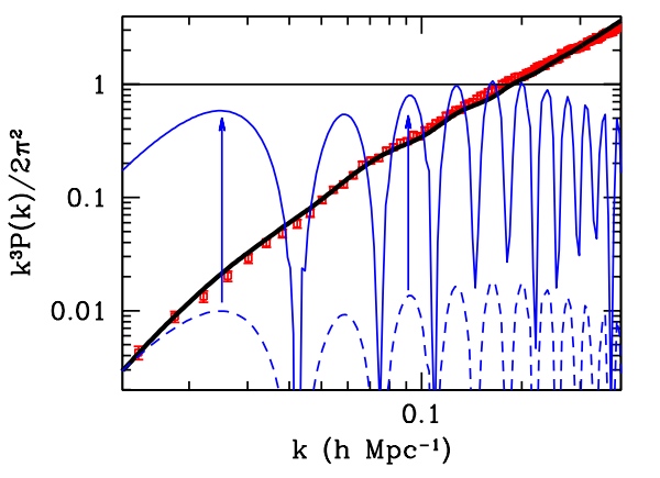
From http://arxiv.org/abs/1112.1320 (Scott Dodelson)
In this plot, the red data points represent actual observation; the black curve, the standard cosmology prediction; and the various blue curves are predictions of (modified) gravity without dark matter.
Let me attempt to explain briefly what this plot represents. It’s all about how matter “clumps” in an expanding universe. Imagine a universe filled with matter that is perfectly smooth and homogeneous. As this universe expands, matter in it becomes less dense, but it will remain smooth and homogeneous. However, what if the distribution of matter is not exactly homogeneous in the beginning? Clumps that are denser than average have more mass and hence, more gravity, so these clumps are more able to resist the expansion. In contrast, areas that are underdense have less gravity and a less-than-average ability to resist the expansion; in these areas, matter becomes increasingly rare. So over time, overdense areas become denser, underdense areas become less dense; matter “clumps”.
Normally, this clumping would occur on all scales. There will be big clumps and small clumps. If the initial distribution of random clumps was “scale invariant”, then the clumping remains scale invariant forever.
That is, so long as gravity is the only force to be reckoned with. But if matter in the universe is, say, predominantly something like hydrogen gas, well, hydrogen has pressure. As the gas starts to clump, this pressure becomes significant. Clumping really means that matter is infalling; this means conversion of gravitational potential energy into kinetic energy. Pressure plays another role: it sucks away some of that kinetic energy and converts it into density and pressure waves. In other words: sound.
Yes, it is weird to talk about sound in a medium that is rarer than the best vacuum we can produce here on the Earth, and over cosmological distance scales. But it is present. And it alters the way matter clumps. Certain size scales will be favored over others; the clumping will clearly show preferred size scales. When the resulting density of matter is plotted against a measure of size scale, the plot will clearly show a strong oscillatory pattern.
Cosmologists call this “baryonic acoustic oscillations” or BAO for short: baryons because they represent “normal” matter (like hydrogen gas) and, well, I just explained why they are “acoustic oscillations”.
In the “standard model” of cosmology, baryonic “normal” matter amounts to only about 4% of all the matter-energy content of the visible universe. Of the rest, some 24% is “dark matter”, the rest is “dark energy”. Dark energy is responsible for the accelerating expansion the universe apparently experienced in the past 4-5 billion years. But it is dark matter that determines how matter in general clumped over the eons.
Unlike baryons, dark matter is assumed to be “collisionless”. This means that dark matter has effectively no pressure. There is nothing that could slow down the clumping by converting kinetic energy into sound waves. If the universe had scale invariant density perturbations in the beginning, it will be largely scale invariant even today. In the standard model of cosmology, most matter is dark matter, so the behavior of dark matter will dominate over that of ordinary matter. This is the prediction of the standard model of cosmology, and this is represented by the black curve in the plot above.
In contrast, cosmology without dark matter means that the only matter that there is is baryonic matter with pressure. Hence, oscillations are unavoidable. The resulting blue curves may differ in detail, but they will have two prevailing characteristics: they will be strongly oscillatory and they will also have the wrong slope.
That, say advocates of the standard model of cosmology, is all the proof we need: it is incontrovertible evidence that dark matter has to exist.
Except that it isn’t. And we have shown that it isn’t, years ago, in our paper http://arxiv.org/abs/0710.0364, and also http://arxiv.org/abs/0712.1796 (published in Class. Quantum Grav. 26 (2009) 085002).
First, there is the slope. The theory we were specifically studying, Moffat’s MOG, includes among other things a variable effective gravitational constant. This variability of the gravitational constant profoundly alters the inverse-square law of gravity over very long distance scales, and this changes the slope of the curve quite dramatically:
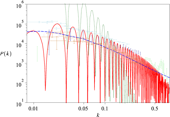
From http://arxiv.org/abs/0710.0364 (J. W. Moffat and V. T. Toth)
This is essentially the same plot as in Dodelson’s paper, only with different scales for the axes, and with more data sets shown. The main feature is that the modified gravity prediction (the red oscillating line) now has a visually very similar slope to the “standard model” prediction (dashed blue line), in sharp contrast with the “standard gravity, no dark matter” prediction (green dotted line) that is just blatantly wrong.
But what about the oscillations themselves? To understand what is happening there, it is first necessary to think about how the actual data points shown in these plots came into existence. These data points are the result of large-scale galaxy surveys that yielded a three-dimensional data set (sky position being two coordinates, while the measured redshift serving as a stand-in for the third dimension, namely distance) for millions of distant galaxies. These galaxies, then, were organized in pairs and the statistical distribution of galaxy-to-galaxy distances was computed. These numbers were then effectively binned using a statistical technique called a window function. The finite number of galaxies and therefore, the finite size of the bins necessarily introduces an uncertainty, a “smoothing effect”, if you wish, that tends to wipe out oscillations to some extent. But to what extent? Why, that is easy to estimate: all one needs to do is to apply the same window function technique to simulated data that was created using the gravity theory in question:
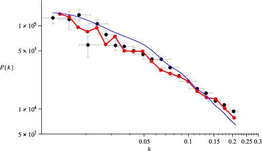
From http://arxiv.org/abs/0710.0364 (J. W. Moffat and V. T. Toth)
This is a striking result. The acoustic oscillations are pretty much wiped out completely except at the lowest of frequencies; and at those frequencies, the modified gravity prediction (red line) may actually fit the data (at least the particular data set shown in this plot) better than the smooth “standard model” prediction!
To borrow a word from the blog post that inspired mine, this is incontrovertible. You cannot make the effects of the window function go away. You can choose a smaller bin size but only at the cost of increasing the overall statistical uncertainty. You can collect more data of course, but the logarithmic nature of this plot’s horizontal axis obscures the fact that you need orders of magnitude (literally!) more data to achieve the required resolution where the acoustic oscillations would be either unambiguously seen or could be unambiguously excluded.
Which leads me to resort to Mark Twain’s all too frequently misquoted words: “The report of [modified gravity’s] death was an exaggeration.”