So a few days ago, Inmarsat and the Malaysian government released what they call the “raw” data about the so-called handshakes between Inmarsat’s Indian Ocean satellite and the ill-fated airliner.
I looked at the data. It was presented in a most inconvenient form, a PDF file with little explanation and with copy-and-paste disabled. Nonetheless, I was able to copy the data to a spreadsheet with only a moderate effort, using Firefox’s built-in PDF viewer instead of Acrobat.
The data set is very detailed, but really, only two columns seem to be of interest: the so-called “beat frequency offset” (BFO) and “burst timing offset” (BTO).
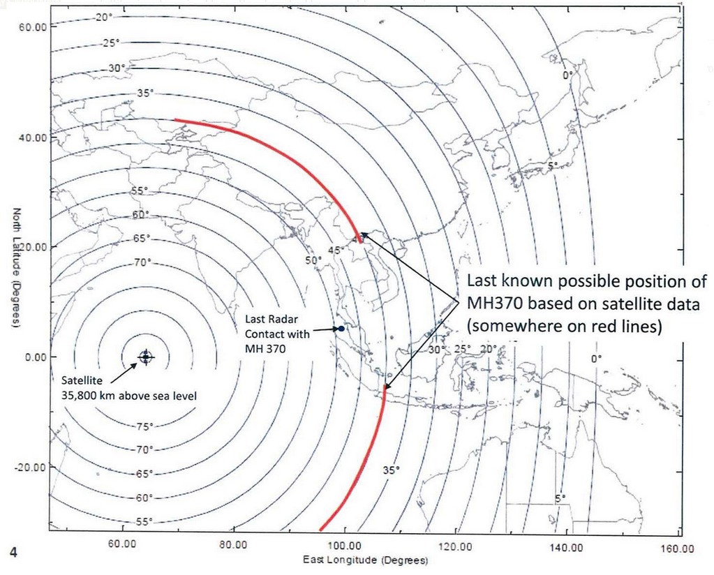
To make a long story short: I am able to confirm the approximate location of the southern search area that was initially explored on March 18 or thereabouts. I am not able to find any rationale for preferring the southerly route over the northern route. The data are symmetrical in this regard. If the airplane flew north, it would have ended up somewhere in Kazakhstan, again in agreement with published predictions for the northerly route.
So here is what I did to arrive at these conclusions.
The little explanation that is offered suggests to me that the BFO is essentially a one-way Doppler frequency shift \((\Delta f)\); whereas the BTO is a two-way propagation delay \((\Delta t)\), with some constant, unknown bias.
The raw data are pretty confusing:
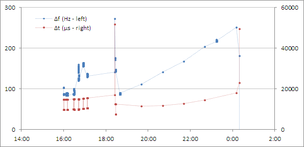
First, there is a lot of stuff happening before and around take-off, around 16:41 UTC. Then something clearly changes around 17:07, the time of the last reported ACARS contact; and once again, there is an anomaly around 18:15, the time of the last reported primary radar contact.
So rightly or wrongly I am summarily dismissing these early data points, as I cannot make heads or tails of them.
Similarly, I am dismissing the very last data points, when clearly some other anomaly was taking place.
Which leaves me with a total of 5 “clean” pairs (both BTO and BFO) of data points between 19:41 and 00:11 UTC. There are two additional data points around 18:15: one is BFO only, the other is BTO only as the corresponding BFO is ambiguous.
My basic assumptions are as follows:
I accept the published time and location of the last civilian (secondary) radar contact (6°55’15” N, 103°34’43” E at 17:21 UTC) and the last military (primary) radar contact (6°49’38” N, 97°43’15” E at 18:15 UTC) as valid. I am assuming that the aircraft flew between these points in a straight line (i.e., along a great circle) at constant speed.
I accept the validity of the aforementioned “clean” Inmarsat data points, 7 in total (2 partial). I am assuming that during this phase of the flight, the aircraft was again traveling in a straight line (that is, along another great circle) at constant speed.
For the sake of simplicity, I assume that the satellite is above the equator, exactly stationary relative to the Earth’s surface, and that the aircraft is not affected by wind. (A more refined calculation might take into account the slight motion of the Inmarsat IOR satellite relative to the ground, and also the known wind patterns at the time of the aircraft’s disappearance. Of course such an analysis is necessarily fraught with significant uncertainties, as not knowing the altitude of the aircraft means we don’t know how it is affected by wind. So the resulting error may not be much smaller than the error I introduced into my calculations by these simplifications.)
The first order of the day was to find a formulation that characterizes the airplane’s trajectory using a minimal number of parameters. For this, I drew the following diagram:
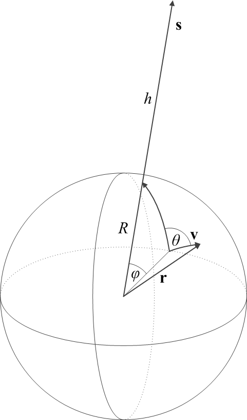
Here, \(R\simeq 6,371~{\rm km}\) is the Earth’s radius; \({\bf s}\) is the geocentric position vector (of length \(R+h\)) of the Inmarsat satellite, which is hovering at an altitude of \(h\simeq 35,800~{\rm km}\); and \(\phi\) is the geocentric angle between the position of the satellite and the initial position of the airplane, which is moving with velocity \({\bf v}\). The angle between the initial velocity vector of the airplane and the direction of the satellite ground track position is given by \(\theta\).
In a Cartesian coordinate system in which the initial position, \({\bf r}(t=t_0)\) of the airplane is given by \({\bf r}_0=[0, 0, R]\) and \({\bf s}\) is in the \(y-z\) plane, these vectors are given by
\begin{align}
{\bf s}&=[0,(R+h)\sin\phi,(R+h)\cos\phi],\\
{\bf r}&=[R\sin\theta\sin\omega t,R\cos\theta\sin\omega t,R\cos\omega t],\\
{\bf v}&=\dot{\bf r}=[v\sin\theta\cos\omega t,v\cos\theta\cos\omega t,-v\sin\omega t],
\end{align}
where the angular velocity is given by \(\omega=v/R\) and of course \(v=|{\bf v}|\).
The distance between the satellite and the airplane is then given by \(d=|{\bf s}-{\bf r}|\). The line-of-sight velocity of the airplane, as seen from the satellite, is given by \(v_{\rm LOS}=({\bf s}-{\bf r})\cdot{\bf v}/d\). This leads us directly to a model of the two Inmarsat observables:
\begin{align}
|\Delta t|&=\left|\frac{2d}{c}\right|,\\
|\Delta f|&=\left|\frac{v_{\rm LOS}}{c}f_0\right|,
\end{align}
where \(c\) is the velocity of light and \(f_0\simeq 1.6435~{\rm GHz}\) is the transmitter frequency on board the aircraft. Absolute values are used to account for the inherent sign ambiguity in the reported observables.
This is not quite the end of the story, however. We know from the description of the Inmarsat data that \(\Delta t\) includes an unknown constant bias \(\Delta t_0\). Furthermore, \(\Delta f\) not only includes an unknown constant bias \(\Delta f_0\) but also includes partial compensation for the Doppler effect by the aircraft transmitter, which we can represent by a scaling factor \(\xi\). Thus the model for the observables must be revised as follows:
\begin{align}
|\Delta t-\Delta t_0|&=\left|\frac{2d}{c}\right|,\\
|\Delta f-\Delta f_0|&=\xi\left|\frac{v_{\rm LOS}}{c}f_0\right|,
\end{align}
This, then, represents our final model for the Inmarsat observables. The model has several adjustable parameters, namely \(v\), \(\phi\), \(\theta\), \(\Delta t_0\), \(\Delta f_0\) and \(\xi\), which can be used to fit the scarce BFO and BTO data points. One question remains, however: shall these be fitted together or separately? Fitting them together would require weighting data of different physical dimenions (seconds for BTO, inverse seconds, or Hz, for BFO). These weights would normally come from estimates of standard deviation on the data, but we have no such estimates. The unknown weights can completely alter the resulting parameter fits, and produce nonsensical results.
Instead, I opted to fit the BFO and BTO data points separately. First, I fitted BTO against \(\Delta t\) by varying only \(v\), \(\phi\), \(\theta\) and \(\Delta t_0\), as the remaining two parameters have no effect on \(\Delta t\). This yielded an estimate for the trajectory of the aircraft. Next, I checked if I can fit \(\Delta f\) against BFO by varying only \(\Delta f_0\) and \(\xi\). (NB: So I am really not fitting the trajectory to the Doppler frequency shift, I am merely checking the validity of the fit. If the model I use is not appropriate to estimate the transmitter frequency bias and Doppler compensation, it might explain why Inmarsat are confident that the northerly route can be excluded.)
Without further ado, the following plot demonstrates the result:
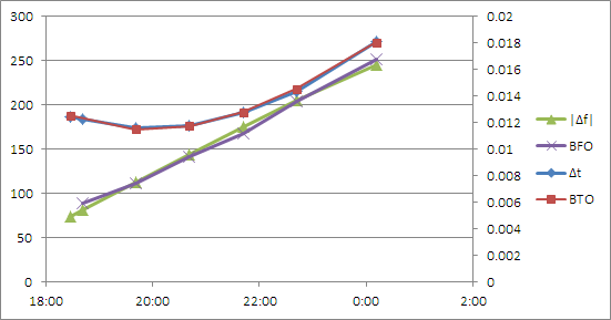
In this plot, the vertical axis on the left is in Hz (for \(|\Delta f|\) and BFO) whereas the vertical axis on the right is in seconds (for \(\Delta t\) and BTO). Yes, I used Microsoft Excel… when you have a nail, a hammer will do nicely.
The values that I obtained for this fit are given by:
\begin{align}
v&=867.16~{\rm kph},\\
\phi&=32.12^\circ,\\
\theta&=-86.55^\circ,\\
\Delta t_0&=0.234572~{\rm s},\\
\Delta f_0&=121.7882~{\rm Hz},\\
\xi&=-0.18199.
\end{align}
This fit by itself does not tell me where the aircraft flew. That is because the model is rotationally symmetric around the ground track position of the Inmarsat satellite. What it does tell me is that at \(t=t_0\) (I arbitrarily chose \(t_0\) to be 19:41 UTC, the time of the first clean Inmarsat data point with both BFO and BTO) the aircraft was on a circle from which the satellite could be seen at 52.6° above the horizon; whereas at the time of the last data point, at 0:11 UTC, the satellite-to-horizon angle was 38.6°.
This is encouraging, as it agrees with published estimates of the infamous “Inmarsat arcs” that position the aircraft along an arc from which the satellite viewing angle is approximately 40°.
But I can do better than this. Let me take a closer look at the two radar data points at 17:21 and 18:15 UTC. These correspond to a great circle trajectory with a velocity of 718.6 kph, almost exactly in the direction of the Inmarsat satellite. By simultaneously extrapolating this trajectory forward and the just calculated Inmarsat-based trajectory backward (for details, see the Wikipedia article on great circle navigation), I can find the time \(t\) when the two trajectories have matching satellite viewing angles. This happens just a few seconds after the last military radar contact at 18:15.
This means that I have an actual starting position for the Inmarsat track at 6°49’34” N, 97°40’47” E, at 18:15:22.7 UTC. If my calculations are valid, at this spot the aircraft would have turned to follow a trajectory that is nearly at a right angle to the line that connects its position to the satellite ground track position.
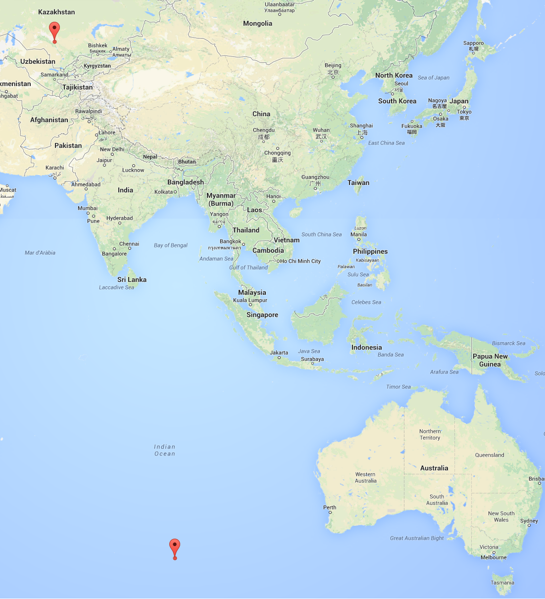
One question, however, remains and it is a nagging one. Did the aircraft turn north or south? Malaysian authorities and Inmarsat insist on the southern track. But I see nothing in the data that they released to support this assertion. If the aircraft turned south, it would have ended up at 38°36’30″S, 88°17’27″E by my calculation, a position that is pretty close to the original search location southwest of Perth, Australia in the Southern Indian Ocean. Therefore, I can confirm the validity of this part of Inmarsat’s analysis.
But what if the airplane flew north instead? That would put it at 44°34’1″N, 66°55’42″E, somewhere in eastern Kazakhstan.
My conclusions, then: the original search area that was designated on March 18, 2014, seems to be validated by the recently released data and my analysis. The assertion that the airplane flew south does not appear to be supported by anything in this data set. If the northern trajectory is not excluded, the airplane may have ended up in Kazakhstan, after flying over places like India, Pakistan, maybe parts of Afghanistan, Uzbekistan and Tajikistan. Is it plausible that such a flight took place without being noticed by these countries’ air defense systems? I’ll leave that for others to decide.
For what it’s worth, here are the two locations that I calculated, presented using Google Maps:
On a final note, I was hesitating before making this blog post public. This is not just a theoretical exercise of matching aircraft trajectories and radio-metric data. There were 239 souls on board, and their relatives still have no idea what happened to them. Is publishing my less than well-informed speculation about the fate of the airliner the right thing to do? I would probably not be publishing anything if my calculations were in contradiction with the “official” analysis. But as I was able to confirm that analysis (again, except for the exclusion of the northern track) it is perhaps not irresponsible for me to publish these results.
The spreadsheet that I used for storing the transcribed Inmarsat data and for my calculations is available for download.